[Paper 리뷰] SimpleSpeech2: Towards Simple and Efficient Text-to-Speech with Flow-based Scalar Latent Transformer Diffusion Models

SimpleSpeech2: Towards Simple and Efficient Text-to-Speech with Flow-based Scalar Latent Transformer Diffusion Models

---

• Non-autoregressive Text-to-Speech model은 duration alignment로 인한 complexity가 있음
• SimpleSpeech2
  • Autoregressive, Non-autoregressive approach를 combine 하여 straightforward model을 구성
  • Simplified data preparation, fast inference, stable generation을 지원
• 논문 (TASLP 2025) : Paper Link

---

1. Introduction

• Text-to-Speech (TTS) model은 크게 autoregressive (AR), non-autoregressive (NAR) model로 구분됨
  • NAR model은 AR model 보다 빠른 생성이 가능하고 robust 하다는 장점이 있지만, fine-grained alignment information에 의존하므로 complexity가 존재함
  • 한편 VALL-E, NaturalSpeech2, NaturalSpeech3 등은 large-scale dataset과 audio codec, language modeling을 활용하여 expressive speech를 생성함
    - BUT, 여전히 efficiency, data requirements 측면에서 한계가 있음

AR-based vs NAR-based TTS

-> 그래서 simple, efficient, stable TTS를 위한 SimpleSpeech2를 제안

 

• SimpleSpeech2
  • 기존 audio codec의 completeness와 compactness를 개선한 Scalar Quantization (SQ)-Codec을 도입
  • DDPM-based diffusion 보다 더 stable 한 Flow-based Scalar Transformer Diffusion을 적용

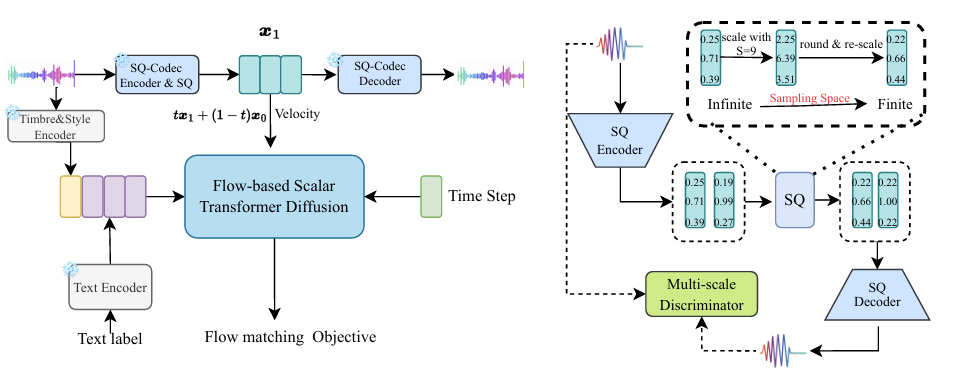
< Overall of SimpleSpeech2 >

• SQ-codec과 flow-based scalar Transformer diffusion을 활용한 simple, stable TTS model
• 결과적으로 기존보다 우수한 성능을 달성

2. Method

• SimpleSpeech2는 크게 3부분으로 구성됨
  • Off-the-Shelf pre-trained text/speaker encoder
    - Speech domain-specific modeling 없이 text/speaker prompt를 encode 하는 역할
  • Pre-trained audio tokenizer
  • LLAMA-style flow-based diffusion Transformer
    

- Text Encoder

• 논문은 large-scale speech-only dataset을 사용하여 TTS system을 training 함
  • 이를 위해 논문은 Automatic Speech Recognition (ASR) model인 Whisper-base를 사용하여 transcript를 얻음
  • 추가적으로 SimpleSpeech를 따라 phoneme과 같은 speech domain-specific knowledge 없이 textual representation을 directly extract 하는 pre-trained ByT5 language model을 도입함

Overview

- Speech Attribute Disentanglement Based Speaker Encoder

• VALL-E와 같이 audio codec에서 speaker prompt representation을 추출하는 경우 recording condition, noise와 같은 acoustic information을 추가적으로 고려해야 함
  • 이를 위해 논문은 pre-trained FACodec을 사용하여 timbre representation을 추출함
  • 먼저 FACodec의 timbre encoder를 통해 global embedding을 추출함
    1. 이후 segment-based average pooling을 사용하여 style vector를 얻음
       - Time에 따른 prosody variation을 반영하기 위해 prompt speech를 3개의 segment로 split 하고 prompt에서 3개의 style vector를 추출함
    2. 최종적으로는 timbre, style vector를 concatenate 하여 사용함

- SQ-Codec

• NaturalSpeech2는 Residual Vector Quantization (RVQ)-based audio codec의 continuous representation을 사용하여 latent diffusion modeling을 수행함
  • BUT, RVQ-basec codec은 다음의 단점이 있음:
    1. RVQ-based codec model을 training 하기 위해서는 complicated design이 필요함
    2. Codebook이 많아지면 LM-based model에 부담을 줄 수 있음
    3. 추출된 continuous representation의 distribution은 complex, infinite 하므로 diffusion modeling이 어려움
  • 이를 해결하기 위해 논문은 RVQ 대신 Scalar Quantization (SQ)을 도입하여 modeling complexity를 줄임
  • 구조적으로 SQ-Codec은 encoder, decoder, scalar quantization으로 구성됨
    1. 먼저 input speech $\mathbf{x}$가 주어지면 encoder는 이를 hidden representation $\mathbf{h}\in\mathcal{R}^{T*d}$로 transfer 함
       - $T,d$ : 각각 frame 수, vector dimension 수
    2. 다음으로 vector $\mathbf{h}_{i}$에 대해 parameter-free scalar quantization module을 적용하여 $\mathbf{h}_{i}$를 fixed scalar space로 quantize 함:
       (Eq. 1) $\mathbf{h}_{i}=\tanh(\mathbf{h}_{i}),\,\,\,\mathbf{s}_{i}=\text{round}(\mathbf{h}_{i}*S)/S$
       - $S$ : scalar space의 scope를 결정하는 hyperparameter
  • (Eq. 1)에서 SQ operation은 $\tanh$ activation을 사용하여 feature value를 $[-1,1]$로 mapping 하고, $\text{round}$ operation을 적용하여 $2*S+1$ range로 scale 함
    - 여기서 해당 value domain을 Scalar Latent Space라고 함

- Flow-based Scalar Latent Transformer Diffusion Models

• Diffusion-based TTS model은 speech data를 continuous space에서 modeling 하지만, compact/complete/finite space가 diffusion modeling에 더 적합함
  - 따라서 논문은 앞선 SQ-Codec을 활용해 noisy distribution을 scalar latent space로 transfer 하고 flow-based diffusion model을 training 함
• Flow-based Diffusion Model
  • SimpleSpeech2는 flow-matching을 활용하여 TTS를 수행함
  • Speech data $\mathbf{x}\sim p(\mathbf{x})$와 Gaussian noise $\epsilon\sim \mathcal{N}(0,I)$가 주어졌을 때 interpolation-based forward process는:
    (Eq. 2) $\mathbf{x}_{t}=\alpha_{t}\mathbf{x}+\beta_{t}\epsilon$
    - $\alpha_{0}=0, \beta_{0}=1,\alpha_{1}=1, \beta_{1}=0,t\in [0,1]$
  • 이때 diffusion과 마찬가지로 $\alpha_{t},\beta_{t}$를 cosine schedule $ \alpha_{t}=\sin(\frac{\pi t}{2}), \beta_{t}=\cos(\frac{\pi t}{2})$ 또는 linear interpolate schedule $\alpha_{t}=t, \beta_{t}=(1-t)$로 설정할 수 있음
    1. 논문은 linear interpolation schedule을 사용하므로 (Eq. 2)는 다음과 같이 얻어짐:
       (Eq. 3) $\mathbf{x}_{t}=t\mathbf{x}+(1-t)\epsilon$
       - $t\in [0,1]$
    2. 대응하는 time-dependent veclocity field는:
       (Eq. 4) $v_{t}(x_{t})=\hat{\alpha}_{t}\mathbf{x}+\hat{\beta}_{t}\epsilon = \mathbf{x}-\epsilon$
       - $\hat{\alpha}_{t},\hat{\beta}_{t}$ : $\alpha,\beta$의 time derivative
  • Velocity field를 가지는 probability flow Ordinary Differential Equation (ODE)는:
    (Eq. 5) $d\mathbf{x}_{t}=\mathbf{v}_{\theta}(\mathbf{x}_{t},t)dt$
    - Velocity $\mathbf{v}$는 neural network $\theta$로 parameterize 됨
  • 여기서 probability flow ODE를 $\epsilon\sim\mathcal{N}(0,I)$에서 backward solve 하면 sample을 생성하고 ground-truth data distribution $p(x)$를 approximate 할 수 있음
    1. BUT, $\mathbf{v}_{\theta}(\mathbf{x}_{t},t)$를 parameterizing 하는 것은 computationally expensive 하므로 $p_{0},p_{1}$ 간의 probability path를 생성하는 vector field $\mathbf{u}_{t}$를 estimate 함
       - 결과적으로 $t=0$에서 $t=1$까지 해당 flow-based generative model을 solve 하면 approximated velocity field $\mathbf{v}_{\theta}(\mathbf{x}_{t},t)$를 사용해 data sample을 얻을 수 있음
    2. Training 시 flow matching objective는 target velocity를 directly regress 함:
       (Eq. 6) $\mathcal{L}_{FM}=\min_{\theta}\mathbb{E}_{t,p_{t}(\mathbf{x})}\left|\left| \mathbf{v}_{\theta}(\mathbf{x},t)-\hat{\alpha}_{t}x-\hat{\beta}_{t}\epsilon\right|\right|^{2}$
       - 이를 Conditional Flow Matching loss라고 함
  • 추가적으로 final output이 scalar latent space에 속하도록 final prediction을 scale 하는 Scalar Quantization (SQ) Regularization을 도입함:
    (Eq. 7) $\hat{\mathbf{x}}=\text{SQ}\left(\theta\left(\epsilon ,T,c\right)\right)$
    - $\theta$ : flow-based Transformer, $\text{SQ}$ : (Eq. 1)의 Scalar Quantization operation

Flow-based Transformer Diffusion

• Architecture
  • SimpleSpeech2는 LLAMA-style Transformer backbone을 활용함 
  • Rotary Position Embedding (RoPE)
    1. RoPE는 relative position을 encoding 할 수 있으므로 long speech generation에 유리함
  • RMSNorm
    1. Training stability를 위해 LayerNorm을 RMSNorm으로 replace 하고 Key-Query Normalization (KQ-Norm)을 Key-Query dot-product attention 이전에 incorportate 함 
    2. KQ-Norm은 attention logit 내의 extremely large value를 eliminate 하여 loss divergence를 방지함
  • Condition Strategy
    1. Condition feature와 noisy latent sequence를 join 하여 self-attention operation에 사용함 
    2. 이를 통해 두 representation이 own space를 가지면서 서로를 고려하도록 함
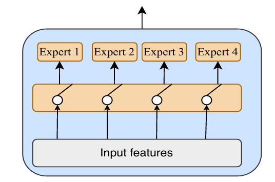
  • Time Mixture-of-Experts
    1. Flow-based diffusion model은 $t\in [0,1]$에서 ODE를 backward solve 하고, scalar latent distribution을 approximate 하는 sample을 생성함
       - Timestep이 $0$에 가까울수록 input $\mathbf{x}$는 highly noisy 하고 timestep이 $1$에 가까울수록 $\mathbf{x}_{t}$에는 semantic information이 포함되어 있음
    2. 여기서 논문은 Flow-based model의 capability를 향상하기 위해 모든 timestep을 $4$ block으로 uniformly divide 하고 각각의 denoising expert에 assign 함 

Time Mixture of Experts

- Classifier-Free Guidance

• Classifier-Free Guidance (CFG)는 generation quality를 향상하는데 효과적임
  • 먼저 CFG를 formulate 하면:
    (Eq. 8) $ \hat{p}(\mathbf{x}|\mathbf{y})=p(\mathbf{x})+\gamma\left(p(\mathbf{x}|\mathbf{y})-p(\mathbf{x})\right)$
    - $\lambda$ : guidance scale
  • CFG는 training 시 conditional distribution $p(\mathbf{x}|\mathbf{y})$와 unconditional distribution $p(\mathbf{x})$를 modeling 함
    1. 추론 시 $\lambda=1$이면 CFG를 사용하지 않고, $\lambda>1$이면 sample의 unconditional likehood를 감소시키고 conditional likelihood를 증가시킴
    2. 특히 CFG는 negative score term을 사용하여 unconditional likelihood를 줄여 sample의 condition information을 masking 함
       - 해당 sample은 unconditional distribution $p(\mathbf{x})$를 optimize 하는 데 사용됨
  • 한편 VoiceCraft는 TTS training을 위해 ASR system의 text transcript를 noisy label로 활용함
    - 이때 해당 noisy label을 활용하는 것은 CFG training stage와 equivalent 하므로 training 시에는 masked sample을 construct 할 필요가 없음
  • Condition $\mathbf{y}$, target $\mathbf{x}$에 대해, generative model이 $p(\mathbf{x}|\mathbf{y})$를 modeling 한다고 하자
    1. Text $\mathbf{y}$가 $n$ word를 포함한다고 하면 $\mathbf{y}$를 $n$ part로 split 할 수 있고, $(\mathbf{y}_{i},\mathbf{x}_{i})$의 correspondence를 얻을 수 있음
       - 이때 TTS는 $\mathbf{y}_{i}, \mathbf{x}_{i}$ 간의 mapping을 학습함
    2. $i\neq j$일 때 $\mathbf{x}_{j}$는 mutually independent 하고 generative model은 distribution $p_{\theta}(\mathbf{x}|\mathbf{y})$를 학습함
    3. 그러면 Bayes formula에 따라 다음을 얻을 수 있음:
       (Eq. 9) $\log p(\mathbf{x}|\mathbf{y})=\log p(\mathbf{y}|\mathbf{x})+\log p(\mathbf{x})-\log p(\mathbf{y})$
    4. $x$의 derivative를 calculate 할 때 last term을 discard 할 수 있으므로:
       (Eq. 10) $\nabla_{x}\log p(\mathbf{x}|\mathbf{y})=\nabla_{x}\log p(\mathbf{y}|\mathbf{x})+\nabla_{x}\log p(\mathbf{x})$
    5. Independence assumption에 따라 $p(\mathbf{y}|\mathbf{x})$를 re-write하면:
       (Eq. 11) $p(\mathbf{y}|\mathbf{x})=p(y_{1},y_{2},...,y_{n}|x_{1},x_{2},...,x_{n})= \prod_{i=1}^{i=n}p(y_{i}|x_{i})$
    6. (Eq. 10), (Eq. 11)을 combine 하면:
       (Eq. 12) $\nabla_{x}\log p(\mathbf{x}|\mathbf{y})=\sum_{i}\nabla_{x}\log p(y_{i}|x_{i})+\sum_{i}\nabla \log p(x_{i})$
  • Large-scale speech dataset에서 input $y_{i}$가 ground-truth label이 아닐 수 있고, 이 경우  $p(y_{i}|x_{i})\rightarrow 0$이 되므로 (Eq. 12)의 first term이 optimization에 contribute 할 수 없음
    1. 극단적으로 text input을 empty로 두고 $p(y_{i}|x_{i})=0$으로 만들 수도 있음
    2. 이 경우 unconditional optimization problem이 됨:
       (Eq. 13) $\nabla_{x}\log p(\mathbf{x}|\mathbf{y})=\sum_{i}\nabla_{x}\log p(x_{i})$

- Sentence Duration

• 논문은 generated speech의 sentence duration을 control 하기 위해 다음의 4가지 방식을 고려함:
  1. ByT5-based Sentence Duration Predictor
     • 아래 그림의 (a)와 같이 pre-trained ByT5 model을 sentence duration prediction model로 사용함
     • 특히 fixed ByT5 model에 learnable attention, linear layer를 add 하고 MSE loss를 통해 training 함
  2. Using Context Learning Ability of ChatGPT
     • (b)와 같이 ChatGPT의 context learning을 활용하여 sentence duration을 얻을 수 있음
     • 이때 ChatGPT는 각 word의 length, pronunciation을 기반으로 coarse sentence duration을 predict 함
       
  3. Using Teacher Model
     • FastSpeech2와 같은 NAR TTS model은 phoneme duration predictor module이 있으므로 각 phoneme의 duration을 얻을 수 있음
     • 이때 diversity를 향상하기 위해 각 phoneme duration에 $[0.9,1.3]$ range의 scale factor를 적용함
  4. Training AR-based Duration Model
     • (d)와 같이 shallow AR-based duration predictor를 training 하여 phoneme/word duration을 autoregressively predict 할 수도 있음

Duration Predictor

3. Experiments

- Settings

• Dataset : Multilingual LibriSpeech
• Comparisons
  - TTS : VALL-E, VoiceCraft, NaturalSpeech2, NaturalSpeech3, E3-TTS, DiTTo-TTS, ARDiT, ChatTTS
  - Speech Tokenizer : EnCodec, DAC, HiFi-Codec, SoundStream

- Results

• 전체적으로 SimpleSpeech2의 성능이 가장 우수함

Model 성능 비교

• MOS 측면에서도 우수한 성능을 보임

Subjective Evaluation

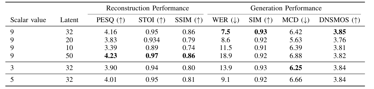
• Speech Tokenizer
  • 논문의 SQ-Codec은 speech tokenizer 중에서 가장 뛰어난 성능을 달성함

Speech Tokenizer

• Tokenizer 성능은 generation performance에도 영향을 미침

Tokenizer 별 성능

• SQ-Codec은 latent $50$, scalar value $9$를 사용했을 때 최적의 성능을 얻을 수 있음

SQ-Codec의 Parameter Setting

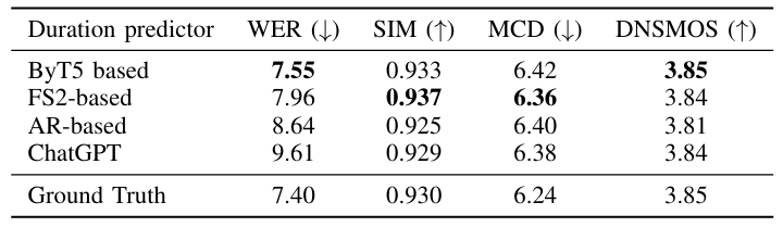
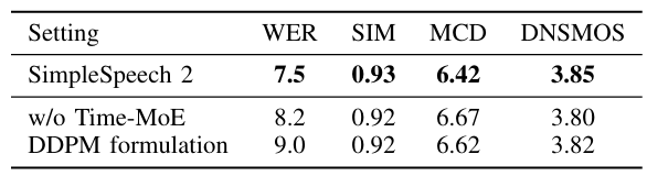
• Ablation Study
  • ByT5 duration predictor를 사용했을 때 가장 낮은 WER을 달성함

Duration Predictor

• Spectrogram 측면에서도 SimpleSpeech2는 다양한 prosody를 합성 가능함

Spectrogram 비교

• 각 component를 제거하는 경우 성능 저하가 발생함

Ablation Study

• CFG scale을 $5$로 설정하면 최적의 결과를 얻을 수 있음

CFG Scale

• Diffusion step이 많을수록 더 나은 성능을 얻을 수 있음

Diffusion Step 별 성능

• Multilingual setting에서도 안정적인 성능을 보임

Multilingual Setting