[Paper 리뷰] Flow2GAN: Hybrid Flow Matching and GAN with Multi-Resolution Network for Few-Step High-Fidelity Audio Generation

Flow2GAN: Hybrid Flow Matching and GAN with Multi-Resolution Network for Few-Step High-Fidelity Audio Generation

---

• Flow Matching 기반의 audio generation model을 추가적으로 개선할 수 있음
• Flow2GAN
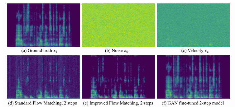
  • Flow matching을 end-point estimation으로 reformulate 하고 perceptually salient quieter region을 emphasize 하기 위해 spectral energy-based loss scaling을 적용
  • 추가적으로 lightweight Generative Adversarial Network fine-tuning과 multi-branch network을 통해 high-fidelity generation을 지원
• 논문 (ICLR 2026) : Paper Link

---

1. Introduction

• Neural vocoding은 mel-spectrogram이나 discrete audio token으로부터 high-resolution waveform을 reconstruct 하는 것을 목표로 함
  • 특히 HiFi-GAN, UnivNet과 같은 Generative Adversarial Network (GAN)-based model은 multi-grained audio detail을 capture 하여 high-fidelity output을 생성할 수 있음
    
  • 한편으로 PriorGrad, RFWave와 같은 diffusion-based model 역시 high-fidelity generation이 가능함
  • BUT, GAN은 mode collapse와 slow convergence로 인한 한계가 있고, diffusion model은 multi-step sampling으로 인한 computational demand의 문제가 있음

-> 그래서 diffusion과 GAN paradigm의 장점만을 combine 한 Flow2GAN을 제안

 

• Flow2GAN
  • Flow matching을 end-point prediction으로 reformulate 하고 low-energy region을 emphasize 하는 spectral energy-based loss를 incorporate
  • Few-step 만으로 audio quality를 refine 하기 위해 GAN fine-tuning과 multi-resolution Fourier coefficient에 대한 multi-branch ConvNeXt structure를 구성

< Overall of Flow2GAN >

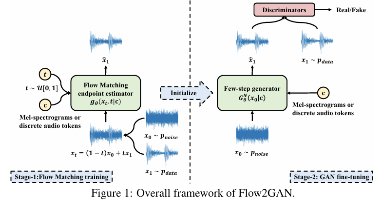
• End-point flow matching과 GAN fine-tuning을 활용한 neural vocoder
• 결과적으로 기존보다 우수한 성능을 달성

2. Preliminary: Flow Matching

• Flow Matching은 noise distribution $p_{noise}=\mathcal{N}(0,I)$를 data distribution $p_{data}$로 transport 하는 velocity field를 학습함
  • Noise point $x_{0}\sim p_{noise}$, data point $x_{1}\sim p_{data}$, $t\sim \mathcal{U}[0,1]$에 대해, linear interpolation $x_{t}=(1-t)x_{0}+tx_{1}$을 사용하여 staright flow path를 정의할 수 있음
    1. 이때 velocity는 $v_{t}=x_{1}-x_{0}$와 같음
    2. Intermediate point $x_{t}$는 서로 다른 $(x_{0},x_{1})$ pair로부터 얻어지고, 각 pair는 distinct velocity $v_{t}$를 생성함
  • 결과적으로 flow matching은 network $f_{\theta}(x_{t},t)$를 training 하여 marginal velocity field를 estimate 함
    1. 즉, $x_{t}$에 condition 된 expected velocity $v(x_{t},t)=\mathbb{E}_{x_{0},x_{1}}\left[v_{t}|x_{t}\right]$와 같음
    2. 이는 randomly sampled pair $(x_{0},x_{1})$에 대해 empirical velocity $v_{t}$를 fitting 하는 것과 equivalent 함:
       (Eq. 1) $ \mathcal{L}_{FM}=\mathbb{E}_{t,x_{0},x_{1}}\left[\left|\left| f_{\theta}(x_{t},t)-v_{t}\right|\right|^{2}\right] $
       
  • 추론 시에는 learned flow model에 대해 $\frac{dx_{t}}{dt}=f_{\theta}(x_{t},t)$에 대해 Ordinary Differential Equation (ODE)를 solve 하여 new data를 sampling 할 수 있음:
    (Eq. 2) $x_{t_{i+1}}=x_{t_{i}}+(t_{i+1}-t_{i})f_{\theta}(x_{t_{i}},t_{i})$
    - 이는 Euler method와 같은 numerical solver를 discrete time step을 통해 approximate 하여 수행됨

3. Method

- Improved Flow Matching for Audio Modeling

• Mel-spectrogram이나 discrete audio token과 같은 compressed acoustic representation $c$에 대해, velocity field는 $f_{\theta}(x_{t},t|c)$와 같이 parameterize 됨
  • BUT, flow matching은 audio modeling시 다음의 한계점이 존재함:
  • Velocity estimation이 어려움
    1. Audio signal은 silent segment나 zero-energy frequency band를 가지므로, model은 해당 region에서 $x_{0}$의 noise를 cancel 하고 empty target $x_{1}$을 recover 할 수 있는 $v_{t}$를 estimate 해야 함
    2. 이로 인해 model은 active region의 difference $v_{t}=x_{1}-x_{0}$ 외에도 empty region에서 $-x_{0}$를 approximate 해야 하므로 learning difficulty가 증가함
  • Loss-Perception Mismatch
    - (Eq. 1)과 같은 Mean Squared Error (MSE) criterion은 모든 signal region에서 prediction error를 uniformly treat 하므로 auditory perception principle과 align 되지 않음
• Reformulation to Endpoint Estimation
  
  • Velocity $v_{t}$ prediction difficulty를 circumvent 하기 위해, 논문은 end-point $x_{1}$을 predict 하도록 $\hat{x}_{1}=g_{\theta}(x_{t},t|c)$와 같이 flow matching을 reformulate 함
  • $v_{t}=\frac{x_{1}-x_{t}}{1-t}$에 대해, (Eq. 1)은 다음과 같이 rewrite 됨:
    (Eq. 3) $\mathcal{L}_{FM} =\mathbb{E}_{t,x_{0},x_{1}}\left[\left|\left| \frac{g_{\theta}(x_{t},t|c)-x_{t}}{1-t}-\frac{x_{1}-x_{t}}{1-t}\right|\right|^{2}\right] =\mathbb{E}_{t,x_{0},x_{1}}\left[ \frac{\left|\left| g_{\theta}(x_{t},t|c)-x_{1}\right|\right|^{2}}{(1-t)^{2}}\right]$
    - 이는 network가 다양한 noise level $(1-t)$의 noisy version $x_{t}$로부터 clean audio $x_{1}$을 reconstruct 하는 것으로 볼 수 있음
  • 이때 (Eq. 3)에서 weighting factor $\frac{1}{(1-t)^{2}}$을 remove 하면 더 나은 성능을 달성할 수 있음:
    (Eq. 4) $\mathcal{L}'_{FM}=\mathbb{E}_{t,x_{0},x_{1}}\left[\left|\left| g_{\theta}(x_{t},t|c)-x_{1}\right|\right|^{2}\right]$
  • 결과적으로 (Eq. 2)의 sampling process는:
    (Eq. 5) $x_{t_{i+1}}=x_{t_{i}}+(t_{i+1}-t_{i})\frac{g_{\theta}(x_{t_{i}},t_{i}|c)-x_{t_{i}}}{1-t_{i}}$
• Spectral Energy-Adaptive Loss Scaling
  • Loss-Perception mismatch를 해결하기 위해, 논문은 reference spectrogram energy에 inversely proportional 하게 flow matching loss를 scale 함
  • 먼저 prediction error는 linear filterbank transformation을 포함한 power STFT $\mathcal{S}(x)=\text{LinFB}(|\text{STFT}(x)|^{2})$에 대해, $\mathcal{S}(g_{\theta}(x_{t},t|c)-x_{1})$과 같이 frequency domain으로 convert 됨
    1. 이후 reference spectrogram energy의 square root $\frac{1}{\sqrt{\mathcal{S}(x_{1})+\epsilon}}$에 대해 element-wise inversely scale 됨
       - $\epsilon=1e-7$
    2. 결과적으로 (Eq. 4)는 다음과 같이 redefine 됨:
       (Eq. 6) $\mathcal{L}^{''}_{FM}=\mathbb{E}_{t,x_{0},x_{1}}\left[\sum_{i,j}\left( \frac{\mathcal{S}(g_{\theta}(x_{t},t|c)-x_{1})}{\sqrt{\mathcal{S}(x_{1})+\epsilon}}\right)_{i,j}\right]$
       - 이때 training stability를 위해 loss scale $\frac{1}{\sqrt{\mathcal{S}(x_{1})+\epsilon}}$을 $0.01$에서 $100$으로 clamp 함

생성된 Mel-Spectrogram 비교

- GAN Fine-Tuning for Refinement and Few-Step Inference

• 논문은 GAN fine-tuning strategy를 활용해 fine-grained audio detail을 개선하고 few-step inference에서 high-fidelity generation을 지원함
  • 이를 위해 (Eq. 5)를 통해 training 된 flow matching model을 $N$ step 동안 forward 하여 few-step GAN generator $G_{\theta}^{N}(x_{0}|c)$를 구성함
    - $N>1$의 $G_{\theta}^{N}(x_{0}|c)$의 경우, gradient는 earlier step의 intermediate output을 end-to-end optimize 할 수 있도록 forward path를 통해 backpropagate 됨
  • 추가적으로 adversarial training을 위해 HiFi-GAN의 Multi-Period Discriminator (MPD)와 UnivNet의 Multi-Resolution Discriminator (MRD)를 도입함
  • 결과적으로 generator는 HingeGAN adversarial loss, $L1$ feature matching loss, multi-scale $L1$ mel-spectrogram reconstruction loss를 통해 fine-tuning 됨

Overview

- Multi-Resolution Network Structure

• Vocos를 따라 논문은 Fourier coefficient를 process 함
  • 특히 audio complexity를 capture 하기 위해 multi-resolution modeling으로 extend 하여 generative modeling에 대한 powerful backbone을 구성함 
  • 구조적으로 Flow2GAN은 서로 다른 resolution의 Fourier coefficient를 process 하는 3개의 branch를 가짐
    1. 먼저 각 branch에서 input signal은 STFT를 통해 transform 되어 complex Fourier coefficient를 생성함
    2. 해당 real/imaginary component는 feature dimension에서 concatenate 된 다음 ConvNeXt block에 전달되어 output complex coefficent를 생성함
    3. 이후 iSTFT를 통해 waveform domain으로 convert 되고, 모든 branch output을 sum하여 final output을 얻음
       - 이때 STFT, iSTFT operation은 differentiable 하므로 전체 model은 end-to-end optimize 됨
  • 추가적으로 mel-spectrogram과 codec token embedding에서 deeper feature를 추출하기 위해, PeriodWave를 따라 모든 branch의 shared condition으로 사용되는 ConvNeXt-based condition encoder를 도입함

Multi-Resolution Network

4. Experiments

- Settings

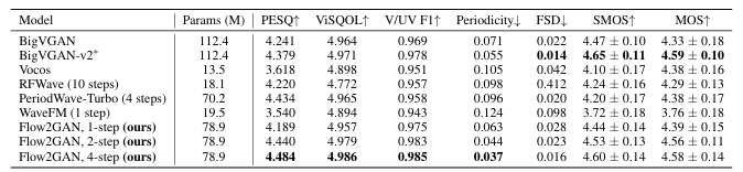
• Dataset : LibriTTS
• Comparisons : BigVGAN, Vocos, RFWave, PeriodWave, WaveFM

- Results

• 전체적으로 Flow2GAN의 성능이 가장 우수함

Model 성능 비교

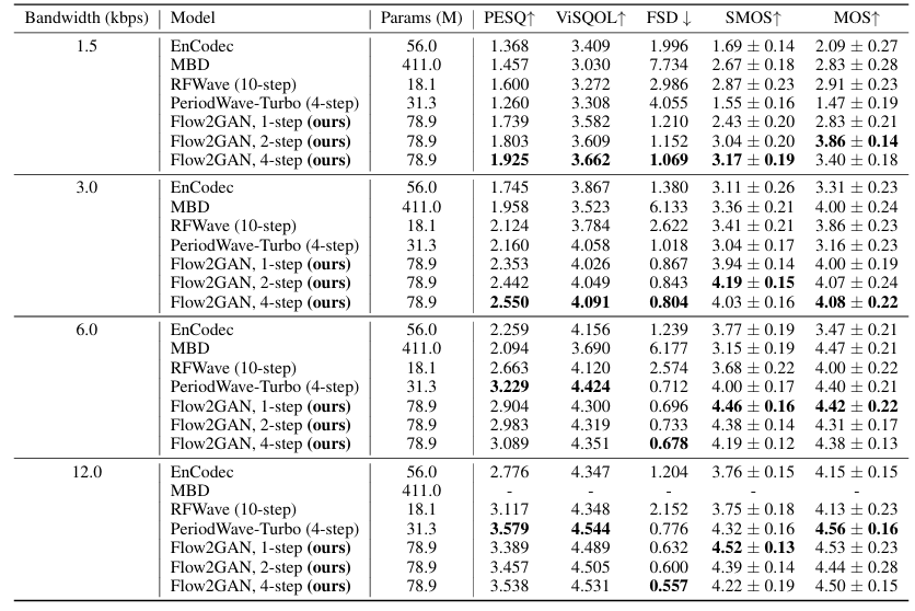
• EnCodec audio token conditioning에 대해서도 뛰어난 reconstruction이 가능함

EnCodec Audio Token Conditioning

• Ablation Study
  • Loss scaling을 flow matching에 적용하면 더 나은 성능을 달성할 수 있음

Ablation Study - Flow Matching

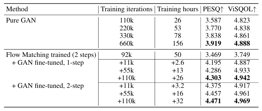
• 2-stage paradigm을 사용하면 기존 GAN 보다 더 나은 성능을 달성할 수 있음

Ablation Study - GAN Training

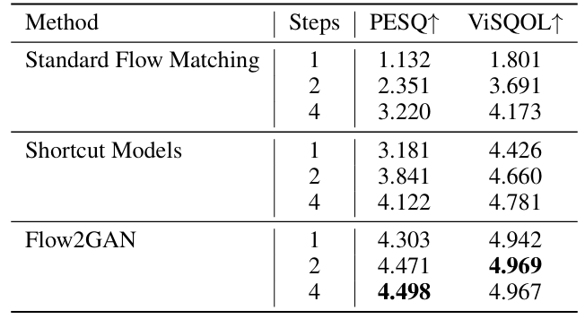
• Flow2GAN은 shortcut model 보다 더 나은 성능을 보임

Ablation Study - Shortcut Model

• Multi-resolution network 역시 성능 향상에 유효함

Ablation Study - Multi-Resolution Network

• Inference Speed
  • Flow2GAN은 Vocos를 제외한 나머지 vocoder 보다 더 빠른 추론 속도를 가짐

Inference Speed

• Zero-Shot TTS
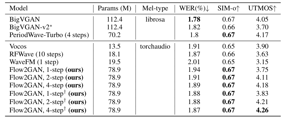
  • Zero-Shot TTS 측면에서도 우수한 성능을 달성함

Zero-Shot TTS