[Paper 리뷰] GLA-Grad++: An Improved Griffin-Lim Guided Diffusion Model for Speech Synthesis

GLA-Grad++: An Improved Griffin-Lim Guided Diffusion Model for Speech Synthesis

---

• Diffusion vocoder는 computational cost와 mismatched distribution에 대한 robustness의 한계가 있음
• GLA-Grad++
  • Griffin-Lim과 reverse process를 integrate 하여 generated signal과 mel-spectrogram 간의 inconsistency를 완화
  • 추가적으로 correction을 적용하여 phase-awareness를 개선
• 논문 (ICASSP 2026) : Paper Link

---

1. Introduction

• WaveGrad, DiffWave와 같은 diffusion-based vocoder는 high-fidelity audio synthesis를 지원함
  • BUT, diffusion-based vocoder는 다음 2가지의 한계점이 있음:
    1. Iterative reverse process로 인한 computational cost
    2. Unseen condition에 대한 robustness
  • 이를 해결하기 위해 PeriodGrad, PeriodWave 등을 고려할 수 있지만 re-training이 필요하다는 단점이 있음
  • 한편으로 GLA-Grad는 Griffin-Lim Algorithm를 reverse process에 integrate 하여 re-training 없이도 mismatched input에 대한 robustness를 향상할 수 있음
    - BUT, GLA-Grad 역시 여전히 multiple iteration step이 필요함

-> 그래서 기존 GLA-Grad의 efficiency를 개선한 GLA-Grad++를 제안

 

• GLA-Grad++
  • Diffusion modeling과 Griffin-Lim Algorithm을 combine하여 spectrogram modeling을 개선
  • Generation 시 correction term을 한 번만 compute 하고 이를 reverse process의 chosen point에 apply 하여 GLA-Grad의 computational burden을 완화

< Overall of GLA-Grad++ >

• Correction term computation을 반영해 기존 GLA-Grad를 개선한 efficient vocoder
• 결과적으로 기존보다 우수한 성능을 달성

2. Background

- Diffusion Models

• Denoising Diffusion Probabilistic Model (DDPM)은 gradual denoising step을 통해 simple noise distribution을 complex data distribution으로 transform 함
  • 먼저 forward process에서 data $\mathbf{y}_{0}$는 Gaussian noise를 통해 progressively corrput 되어 nearly isotropic Gaussian noise $\mathbf{y}_{T}$로 transform 됨:
    (Eq. 1) $ q(\mathbf{y}_{t}|\mathbf{y}_{t-1})=\mathcal{N}(\mathbf{y}_{t};\sqrt{1-\beta_{t}}\mathbf{y}_{t-1}, \beta_{t}I)$
    - $\beta_{t}$ : step $t$에서 noise level을 control 하는 역할
    
  • $\mathbf{y}_{0}$에서 (Eq. 1)을 iteratively apply 하는 대신, 다음과 같이 simplify 할 수 있음:
    (Eq. 2) $\mathbf{y}_{t}=\sqrt{\bar{\alpha}_{t}}\mathbf{y}_{0}+\sqrt{1-\bar{\alpha}_{t}}\epsilon,\,\,\, \epsilon\sim\mathcal{N}(0,I)$
    - $\alpha_{t}=1-\beta_{t},\bar{\alpha}_{t}=\prod_{s=1}^{t}\alpha_{s}$
  • Reverse process는 $\mathbf{y}_{t}$를 denoise 하여 $\mathbf{y}_{0}$를 recover 함:
    (Eq. 3) $\mathbf{y}_{t-1}=\frac{1}{\sqrt{\alpha}_{t}}\left(\mathbf{y}_{t}-\frac{1-\alpha_{t}}{\sqrt{ 1-\bar{\alpha}}_{t}}\epsilon_{\theta}(\mathbf{y}_{t},t)\right) +\sigma_{t}\mathbf{z},\,\,\, \mathbf{z}\sim \mathcal{N}(0,I)$
    - $\epsilon_{\theta}(\mathbf{y}_{t},t)$ : $\mathbf{y}_{t}$의 noise를 predict 하는 neural network, $\sigma_{t}=\sqrt{\frac{1-\bar{\alpha}_{t-1}}{1-\bar{\alpha}_{t}}\beta_{t}}$: added Gaussian noise의 variance를 control 하는 역할
  • Training objective는 predicted noise에 대한 simplified Mean-Squared Error loss를 사용함:
    (Eq. 4) $\mathcal{L}_{DDPM}=\mathbb{E}_{\mathbf{y}_{0},\epsilon\sim\mathcal{N}(0,I),t}\left[ \left|\left| \epsilon-\epsilon_{\theta}(\mathbf{y}_{t},t)\right|\right|_{2}^{2}\right]$
  • 이때 WaveGrad는 mel-spectrogram에 condition 된 DDPM-based vocoder로써,
    1. Loss에 $L_{1}$ norm을 적용한 다음의 denoising equation을 사용함:
       (Eq. 5) $\mathbf{y}_{t-1}=\frac{1}{\sqrt{\alpha}_{t}}\left(\mathbf{y}_{t}-\frac{1-\alpha_{t}}{\sqrt{1-\bar{\alpha}_{t}}}\epsilon_{\theta} (\mathbf{y}_{t},\tilde{\mathbf{X}},\sqrt{\bar{\alpha}_{t}})\right) +\sigma_{t}\mathbf{z}$
       - $\tilde{\mathbf{X}}$ : conditioning mel-spectrogram

- Griffin-Lim Algorithm

• Griffin-Lim Algorithm (GLA)는 phase information이 unavailable 할 때 magnitude spectrogram으로부터 time-domain signal을 iteratively reconstruct 함
  • 즉, phase를 iteratively refining 하여 STFT magnitude가 주어진 spectrogram과 match 되는 signal을 estimate 함
  • Target magnitude spectrogram $|X(\omega, t)|$, signal $x[n]$의 STFT $\mathcal{G}\{x[n]\}$에 대해, GLA는 다음의 2가지 projection step을 alternate 함:
    
    1. Projection onto the Magnitude Constraint
       - Iteration $k$의 complex STFT estimate $Y_{k}(\omega, t)$에 대해 updated STFT는 current phase를 preserve 하면서 magnitude를 target magnitude로 replace 함:
       (Eq. 6) $Y'_{k}(\omega, t)=|X(\omega,t)|\frac{Y_{k}(\omega, t)}{|Y_{k}(\omega, t)|}$
    2. Projection onto the Time-domain Consistency
       - Modified STFT를 iSTFT를 통해 time-domain으로 convert 하고 resulting signal의 STFT를 recompute 하여 overlapping frame 간의 consistency를 enforce 함:
       (Eq. 7) $Y_{k+1}(\omega,t)=\mathcal{G}\left\{ \mathcal{G}^{-1}\{ Y'_{k}(\omega, t)\}\right\}$
  • 결과적으로 GLA는 random phase로 initialize 된 다음, converge 할 때까지 iterate 되어 STFT magnitude가 target $|X(\omega, t)|$를 approximate 하는 time-domain signal $x[n]$을 생성함

3. Method

• Reverse process는 random Gaussian noise를 iteratively denoise 하여 waveform을 생성함
  • Early iteration 시 iterative sample $\mathbf{y}_{t}$는 highly noisy 하므로 (Eq. 5)는 다음과 같이 reformulate 됨:
    (Eq. 8) $\mathbf{y}_{t-1}=\sqrt{\bar{\alpha}_{t-1}}\underset{\text{predicted}\,\,\mathbf{y}_{0}}{\underbrace{\left( \frac{\mathbf{y}_{t}-\sqrt{1-\bar{\alpha}_{t}}\epsilon_{\theta}(\mathbf{y}_{t},\tilde{\mathbf{X}},\sqrt{\bar{\alpha}_{t}}) }{\sqrt{\bar{\alpha}_{t} }}\right)}} +\underset{\text{direction pointing to}\,\,\mathbf{y}_{t}}{\underbrace{\sqrt{1-\bar{\alpha}_{t-1}-\sigma_{t}^{2}}\cdot \epsilon_{\theta}(\mathbf{y}_{t},\tilde{\mathbf{X}}, \sqrt{\bar{\alpha}_{t}}) }}+\underset{\text{random noise}}{\underbrace{\sigma_{t}\mathbf{z}}}$
    - First term은 denoised estimate/predicted $\mathbf{y}_{0}$를 rescale 하고, second term은 current step에서 predicted noise의 contribution을 나타내고, third term은 controlled stochasticity를 reintroduce 함
  • 이를 기반으로 논문은 denoising process의 early iteration 시 predicted $\mathbf{y}_{0}$를 accurate estimate로 replace 하여 waveform generation을 개선함

Overview

- Magnitude Spectrogram Estimation

• Model은 mel-spectrogram $\tilde{\mathbf{X}}$에 condition 되고, 이는 magnitude spectrogram $\mathbf{X}$의 lossy representation으로 볼 수 있음
  • 이때 $\tilde{\mathbf{X}}$는 $\tilde{\mathbf{X}}=\mathbf{BX}$와 같이 얻어짐
    - $\mathbf{B}\in\mathbb{R}_{+}^{M\times F}$ : mel-filterbank matrix, $F$ : frequency bin 수, $M<F$ : mel-band 수
  • 이후 mel-spectrogram으로부터 magnitude spectrogram을 reconstruct 하기 위해 mel-filterbank의 pseudo-inverse를 $\tilde{\mathbf{X}}:\hat{\mathbf{X}}=\mathbf{B}^{+}\tilde{\mathbf{X}}$와 같이 적용함

- Phase Recovery

• Magnitude spectrogram의 phase estimation은 GLA를 사용하여 얻어짐
  • 이때 current iterate의 phase를 사용하는 기존 GLA-Grad와 달리 논문은 random initialization을 사용함
    - Early iteration의 phase information은 unreliable 하고 GLA convergence에 거의 영향을 미치지 않기 때문
  • 따라서 GLA-Grad++에서 GLA는 diffusion process와 independent 하고 denoising 이전에 한 번만 적용됨
  • Magnitude, phase reconstruction 이후, iSTFT를 사용하여 time-domain signal $\tilde{\mathbf{x}}$를 reconstruct 함
    1. 이를 위해 GLA-Grad와 같이 2-stage generation을 수행하는 대신, first stage에서는 전체 $\mathbf{y}_{t}$를 update 하지 않고 initial step에서 (Eq. 8)의 predicted $\mathbf{y}_{0}$ term을 $\tilde{\mathbf{x}}$로 replace 함:
       (Eq. 9) $\mathbf{y}_{t-1}=\sqrt{\bar{\alpha}_{t-1}}\tilde{\mathbf{x}} +\sqrt{1-\bar{\alpha}_{t-1}-\sigma_{t}^{2}}\cdot \epsilon_{\theta}\left(\mathbf{y}_{t},\tilde{\mathbf{X}},\sqrt{\bar{\alpha}_{t}}\right) +\sigma_{t}\mathbf{z}$
    2. 이후 second stage에서는 (Eq. 8)의 standard denoising equation을 사용함

4. Experiments

- Settings

• Dataset : LJSpeech, VCTK
• Comparisons : WaveGrad, GLA-Grad

- Results

• 전체적으로 GLA-Grad++의 성능이 가장 우수함

Model 성능 비교

• GLA-Grad++는 GLA-Grad 보다 더 빠른 추론 속도를 보임

추론 속도 비교

• Oracle Result
  • Correct phase를 사용하는 것이 correct magnitude spectrogram을 사용하는 것보다 더 효과적임

Oracle Result

• Impact of the End Timestep
  • Timestep 2를 사용했을 때 최적의 결과를 달성함

End-point 별 성능 (LJSpeech)

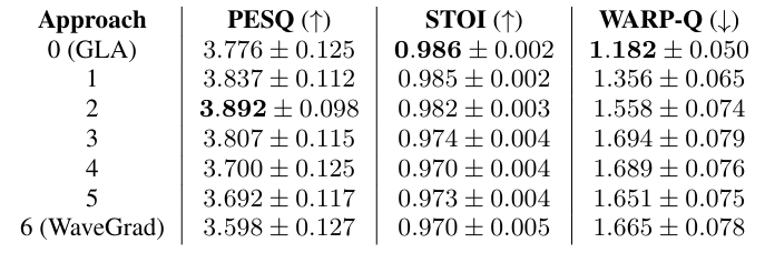
• VCTK datset에서도 마찬가지의 결과를 보임

End-point 별 성능 (VCTK)

• 실제로 각 test file에 대해 global optimal timestep은 2로 나타남

Optimal Timestep