[Paper 리뷰] LangWave: Realistic Voice Generation based on High-Order Langevin Dynamics

LangWave: Realistic Voice Generation based on High-Order Langevin Dynamics

---

• Diffusion model은 음성 생성에서 우수한 성능을 보이고 있지만 대부분 first-order stochastic differential equation이나 equivalent diffusion model에 의존함
• LangWave
  • 기존의 first-order method에서 벗어나 third-order Langevin dynamical system을 활용하여 waveform을 생성
  • Ambient Euclidean space에서 voice wave diffusion, position, velocity, acceleration을 동시에 모델링하여 white noise에서 waveform으로의 wave evolution을 보다 정확하게 control 함
• 논문 (ICASSP 2024) : Paper Link

---

1. Introduction

• 음성 생성을 위해 flow-based, variation autoencoder (VAE), generative adversarial network (GAN) 등이 활용되고 있음
  • 특히 최근의 score-based generative model (SGM)은 뛰어난 합성 품질을 보이고 있음
    - 여기서 scroe는 target data 분포의 high-density area를 가리키는 gradient를 의미하고, score가 가리키는 direction을 따라 target 분포와 유사한 sample wave를 얻는 방식으로 동작함
  • BUT, SGM을 사용하는 기존의 vocoder들은 대부분 first-order stochastic differential equation (SDE)를 기반으로 함
    - 대표적으로 DiffWave나 PriorGrad는 모두 variance preserving SDE의 discrete form인 denoising diffusion probabilistic model (DDPM)을 사용
    - 이러한 first-order SDE는 position만 describe 하고 velocity나 acceleration은 모델링하지 않는 한계가 있음

-> 그래서 diffusion 과정에서 waveform의 position 뿐만 아니라 velocity, acceleration 등을 모델링할 수 있는 third-order Langevin dynamics를 활용하는 LangWave를 제안

 

• LangWave
  • Third-order Langevin dynamics (TOLD)는 desired stationary 분포를 가지고 first-order SDE보다 빠르게 수렴하는 것이 증명되어 있음
    - 따라서 LangWave는 white noise와 waveform 간의 diffusion과 sampling을 위해 TOLD를 적용하여 vocoder 작업을 개선함
  • 이때 TOLD의 적용을 위해 3가지 variable set을 활용
    - Data point의 position을 나타내는 variable set
    - 각각 voice wave의 velocity, acceleration을 모델링하는 variable set
  • 위 3가지의 variable set를 서로 결합하여 position-velocity, velocity-acceleration에 대한 Hamiltonian system을 구성
    - 이와 같이 구성된 두 Hamiltonian system을 통해 TOLD의 mixing time과 expressiveness를 향상 가능

< Overall of LangWave >

• First-order SDE에서 벗어나 TOLD를 기반으로 하는 새로운 음성 생성 paradigm을 제시
• Sampling process 동안 ambient space에서 position, velocity, acceleration을 동시에 모델링하여 generation path를 smooth 하게 만들고 더 빠르게 target 분포에 도달할 수 있도록 함
• 결과적으로 기존 모델들보다 우수한 성능을 달성

2. Method

- Third-order Langevin Dynamics

• Langevin diffusion에 대한 first-order discretization은 generative model에서 성공적으로 사용되고 있음
  • 한편으로 이를 high-order scheme으로 확장하는 것을 고려해 볼 수 있고, 특히 third-order Langevin dynamics (TOLD)는 수렴성에 대한 이론적 증명이 확립되어 있음 
  • 따라서 논문은 TOLD를 음성 생성에 적용하기 위해 다음과 같이 parameter를 설정함:
    (Eq. 1) $\left\{\begin{matrix}
    d\mathbf{q}_{t}=\mathbf{p}_{t}dt \\
    d\mathbf{p}_{t}=-\mathbf{q}_{t}dt+\gamma\mathbf{s}_{t}dt \\
    d\mathbf{s}_{t}=-\gamma\mathbf{p}_{t}-\xi\mathbf{s}_{t}dt+\sqrt{2\xi L^{-1}}d\mathbf{w}_{t}
    \end{matrix}\right.$
  • 여기서 LangWave는 $\mathbf{q}, \mathbf{p},\mathbf{s}$가 음성이 ambient space에서 diffusion 되고 sampling 될 때 각각 음성의 position, velocity, acceleration을 나타낸다고 가정 
    - Position의 derivative는 velocity이고, velocity의 derivative는 acceleration이기 때문
    - $\gamma, \xi, L$ : hyperparameter로 논문에서는 $\xi=6, \gamma=\sqrt{10}$으로 설정
    - $\mathbf{w}_{t}$ : standard Wiener process
  • TOLD는 linear SDE로써, $\mathbf{x}_{t}=(\mathbf{q}_{t},\mathbf{p}_{t}, \mathbf{s}_{t})^{\top}\in\mathbb{R}^{3d}$라고 했을 때 (Eq. 1)은 다음의 compact form으로 나타낼 수 있음:
    (Eq. 2) $d\mathbf{x}_{t}=f(t)\mathbf{x}_{t}dt+G(t)d\mathbf{w}_{t},\,\,\, t\in[0,T]$
    - 여기서,
    (Eq. 3) $f(t):=\begin{pmatrix}
    0 & 1 & 0 \\
    -1 & 0 & \sqrt{10} \\
    0 & -\sqrt{10} & -6 \\
    \end{pmatrix}\otimes \mathbf{I}_{d}$
    (Eq. 4) $G(t):=\begin{pmatrix}
    0 & 0 & 0 \\
    0 & 0 & 0 \\
    0 & 0 & \sqrt{12L^{-1}} \\
    \end{pmatrix}\otimes \mathbf{I}_{d}$
    - $\mathbf{I}_{d}$ : $d$-dimensional identity matrix, $\otimes$ : Kronecker product

- Perturbation Kernel

• (Eq. 1)에서 정의된 TOLD는 original 음성 분포의 velocity, acceleration을 destory 하고 white noise로 변환하는 forward process 
  • 이때 conditional input인 mel-spectrogram 하에서 white noise를 waveform으로 변환하기 위해서는 기존의 first-order SDE와는 완전히 다른 score를 구해야 함
    - 여기서 score는 각 moment에서 TOLD의 marginal probability density와 관련되어 있으므로, 서로 다른 moment의 density에 대한 transition을 구할 수 있다면 white noise에서 음성으로의 변환을 달성할 수 있음
  • 따라서 TOLD에 대한 solution process $\mathbf{x}_{t}$의 transition density $p(\mathbf{x}_{t}| \mathbf{x}_{0})$는 Fokker-Planck-Kolmogorov (FPK) equation의 해와 같음:
    (Eq. 5) $\frac{\partial p(\mathbf{x}_{t},t)}{\partial t}=-\sum_{t=1}^{d}\frac{\partial[(f(t)\mathbf{x}_{t})_{i}p(\mathbf{x}_{t},t)]}{\partial x_{i}} + \sum_{i=1}^{d}\sum_{j=1}^{d}\frac{\partial^{2}}{\partial x_{i}\partial x_{j}}[(G(t)G(t)^{\top})_{i,j}p(\mathbf{x}_{t},t)]$
    - $(f(t)\mathbf{x}_{t})_{i}$ : vector $f(t)\mathbf{x}_{t}$의 $i$-th element
    - $(G(t)G(t)^{\top})_{i,j}$ : matrix $G(t)G(t)^{\top}$의 $i$-th row, $j$-th column의 element
  • 이때 $p(\mathbf{x}_{t}| \mathbf{x}_{0})$는 다음의 ordinary differential equation (ODE)를 만족하는, 평균 $\mu_{t}$, 분산 $\Sigma_{t}$를 가지는 Gaussian:
    (Eq. 6) $\frac{d\mu_{t}}{dt}=f(t)\mu_{t}$
    (Eq. 7) $\frac{d\Sigma_{t}}{dt}=f(t)\Sigma_{t}+[f(t)\Sigma_{t}]^{\top}+G(t)G(t)^{\top}$
  • 위 ODE array를 solve 하면:
    (Eq. 8) $\mu_{t}=\exp\left[\int_{0}^{t}f(\tau)d\tau\right]\mu_{0}$
    (Eq. 9) $\Sigma_{t}=\exp\left[\int_{0}^{t}f(\tau)d\tau\right]\Sigma_{0}\exp\left[\int_{0}^{t}f(\tau)d\tau\right]^{\top}+\int_{0}^{t}\exp\left[\int_{s}^{t}f(\tau)d\tau\right]G(s)G(s)^{\top}\exp\left[\int_{s}^{t}f(\tau)d\tau\right]^{\top}ds$
  • 여기서 $t$를 무한대로 두면, prior 분포를 얻을 수 있음:
    (Eq. 10) $p_{\infty}(\mathbf{x})=\mathcal{N}(\mathbf{q};0_{d},L^{-1}\mathbf{I}_{d})\mathcal{N}(\mathbf{p};0_{d},L^{-1}\mathbf{I}_{d})\mathcal{N}(\mathbf{s};0_{d},L^{-1}\mathbf{I}_{d})$
  • 그러면 $\nabla_{\mathbf{x}_{t}}\log$ operation으로 target score를 얻을 수 있음:
    $\nabla_{\mathbf{x}_{t}}\log p(\mathbf{x}_{t}| \cdot)=-\nabla_{\mathbf{x}_{t}}\frac{1}{2}(\mathbf{x}_{t}-\mu_{t})\Sigma^{-1}_{t}(\mathbf{x}_{t}-\mu_{t})= -\Sigma^{-1}_{t}(\mathbf{x}_{t}-\mu_{t})$
    $\,\,\,\,\,\,\,\,\,\,\,\,\,\,\,\,\,\,\,\,\,\,\,\,\,\,\,\,\,\,\,\,\,\,\,\,\,= -L_{t}^{-\top}L_{t}^{-1}(\mathbf{x}_{t}-\mu_{t}) = -L_{t}^{-\top}\epsilon_{3d}$
    - $\epsilon_{3d} \sim \mathcal{N}(0,\mathbf{I}_{3d})$ : Cholesky factorization, $\Sigma_{t} = L_{t}L_{t}^{\top}$ : $\Sigma_{t}$의 covariance matrix
    - 결과적으로 $\mathbf{x}_{t}$는 $\mathbf{x}_{t}=\mu_{t}+L_{t}\epsilon$의 reparameterization을 통해 sampling됨

- The Objective

• $p(\mathbf{x}_{0})$는 생성하고자 하는 initial velocity, acceleration을 가지는 target audio의 분포를 나타내고, $p(\mathbf{x}_{0})$는 (Eq. 1)의 TOLD를 따라 $p(\mathbf{x}_{t})$를 통해 $p(\mathbf{x}_{T})$로 diffuse 됨 
  • 여기서 생성 과정의 목표는 해당 process를 reverse 하는 model을 학습시키는 것
    - Prior probability의 approximation $q(\mathbf{x}_{T})$에서 sampling 한 다음, $q(\mathbf{x}_{t})$를 통해 $q(\mathbf{x}_{0})$의 denoising인 time-reverse TOLD를 수행함
  • 결과적으로 LangWave의 목표는 $q(\mathbf{x}_{0})$와 $p(\mathbf{x}_{0})$ 간의 차이를 최대한 작게 만드는 것으로, 다음의 Kullback-Leibler (KL) divergence를 활용함:
    $D_{KL}(p_{0}||q_{0})=-\int_{0}^{T}\frac{\partial D_{KL}(p_{t}||q_{t})}{\partial t}dt +D_{KL}(p_{T}||q_{T})$
  • $T$가 크면 $D_{KL}(p_{T}||q_{T})$는 무시할 수 있을 만큼 작으므로, objective 계산에서 가장 중요한 것은 $\int_{0}^{T}\frac{\partial D_{KL}(p_{t}||q_{t})}{\partial t}dt$의 값을 계산하는 것
    - 이는 다음의 propsition으로 유도됨:
    
    [Proposition 2.1.]
    모든 moment에서 marginal distribution 간의 KL distance의 derivative는 acceleration score 간의 차이를 적분하여 얻을 수 있다. 즉,
    $\frac{\partial D_{KL}(p_{t}||q_{t})}{\partial t}=-\frac{6}{L}\int p(\mathbf{x}_{t})||\nabla_{\mathbf{s}_{t}}\log p(\mathbf{x}_{t})-\nabla_{\mathbf{s}_{t}}\log q(\mathbf{x}_{t})||_{2}^{2}d\mathbf{x}_{t}$
    그리고,
    $D_{KL}(p_{0}||q_{0})=\mathbb{E}_{t\sim\mathcal{U}[0,T],\mathbf{x}_{t}\sim p(\mathbf{x}_{t})}\left[|| \nabla_{\mathbf{s}_{t}}\log p(\mathbf{x}_{t})-\nabla_{\mathbf{s}_{t}}\log q(\mathbf{x}_{t})||_{2}^{2}\right]$
    
    
  • 여기서 LangWave는 score $\nabla_{\mathbf{s}_{t}}\log p(\mathbf{x}_{t})$를 추정하기 위해 neural network를 활용함
    
  • 그러면 $\mathfrak{S}_{\theta}(\mathbf{x}_{t},t)$를 score model이라고 했을 때, 전체 initial auxiliary signal $\mathbf{q}, \mathbf{s}$에 대해 marginalizing 하여 acceleration score matching (ASM)을 얻을 수 있음:
    (Eq. 11) $\mathcal{L}_{ASM}:=\mathbb{E}_{t\sim\mathcal{U}[0,T]}\left[\lambda(t)\mathbb{E}_{\mathbf{q}_{0}\sim p(\mathbf{q}_{0}), \mathbf{x}_{t}\sim p(\mathbf{x}_{t}| \mathbf{q}_{0})} || \nabla_{\mathbf{s}_{t}}\log p(\mathbf{x}_{t}| \mathbf{q}_{0})-\mathfrak{S}_{\theta}(\mathbf{x}_{t},t) ||_{2}^{2}\right]$
    - 이때 해당 ASM이 correct loss임을 보여주는 다음의 proposition이 존재함:
    
    [Proposition 2.2.]
    (Eq. 11)의 ASM은 score matching (SM), denoising score matching (DSM)과 동치이다.

- Sampling with LangWave and Network Structure

• Score $\nabla_{\mathbf{s}_{t}} \log p(\mathbf{x}_{t})$에 대한 optimal predictor $\mathfrak{S}_{\theta}(\mathbf{x}_{t},t)$를 얻은 다음, prior 분포를 target wave로 denoise 하기 위해 backward TOLD와 연결할 수 있음
  • 그러면 backward TOLD는 다음과 같이 근사됨:
    (Eq. 12) $ \left\{\begin{matrix}
    d\mathbf{q}_{t} =-\mathbf{p}_{t}dt \\
    d\mathbf{p}_{t} =\mathbf{q}_{t}dt-\gamma\mathbf{s}_{t}dt \\
    d\mathbf{s}_{t} =\gamma\mathbf{p}_{t}dt+\xi\mathbf{s}_{t}dt+2\xi L^{-1}\mathfrak{S}_{\theta}(\mathbf{x}_{t},t)dt+\sqrt{2\xi L^{-1}}d\bar{\mathbf{w}}_{t}
    \end{matrix}\right.$
    - 이를 통해 discretize 된 다음, waveform sampling에 사용됨
  • Score prediction network $\mathfrak{S}_{\theta}$는 아래 그림과 같이 구성되고, wave (noise)와 해당 velocity, acceleration을 input으로 함
    - 추가적으로 time, mel-spectrogram에 대한 condition input을 사용하고, score $\nabla_{\mathbf{s}_{t}}\log p(\mathbf{x}_{t}| \mathbf{q}_{0})$를 output 함

Score Prediction Network

3. Experiments

- Settings

• Dataset : LJSpeech
• Comparisons : FloWaveNet, ItoWave, WaveGlow, DiffWave

- Results

• MOS 측면에서 LangWave는 다른 모델들보다 더 뛰어난 성능을 보임

주관적 품질 비교

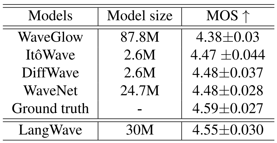
• 정량적 지표 측면에서도 LangWave는 가장 우수한 성능을 보임

정량적 성능 비교

• Ablation Study
  • Generation step이 많을수록 생성되는 sample의 품질은 좋아짐
  • BUT, $T=50$일 때의 MOS도 $T=500$일 때와 비교하여 충분히 우수한 것으로 나타남 (0.2 차이)

Sampling Step 별 성능

• 한편으로 LangWave는 ItoWave에 비해 더 적은 mixing time을 가짐
  - 실제로 서로 다른 time step에서 생성된 waveform을 비교해 보면, LangWave가 ItoWave보다 우수한 품질을 보임

Time Step에 따른 ItoWave와의 비교