[Paper 리뷰] PriorGrad: Improving Conditional Denoising Diffusion Models with Data-Dependent Adaptive Prior

PriorGrad: Improving Conditional Denoising Diffusion Models with Data-Dependent Adaptive Prior

---

• Denoising diffusion probabilistic model은 data densitiy의 gradient를 추정하여 고품질의 sample을 생성할 수 있음
• 일반적으로 prior noise를 standard Gaussian 분포로 정의하지만, 해당하는 data 분포는 더 복잡할 수 있음
  - Data와 prior 사이의 discrepancy로 인해 data sample에서 prior noise를 제거하는 것이 어려워짐
• PriorGrad
  • Conditional information 기반의 data statistics로부터 도출된 adaptive prior를 적용하여 conditional diffusion model을 향상
  • PriorGrad를 음성 합성에 적용하여 더 빠른 수렴 및 합성 품질을 달성
• 논문 (ICLR 2022) : Paper Link

---

1. Introduction

• Denoising Diffusion Probabilistic Model (DDPM)은 high-fidelity의 sample을 합성하는데 우수한 성능을 보임
  • 음성 합성에서 diffusion model은 text, spectral information에 따라 condition 된 spectral, time-domain audio를 합성함
  • BUT, diffusion model은 고품질의 audio를 생성할 수 있지만 비효율성이 잠재되어 있음
    - Reverse diffusion process를 학습하기 어렵고 느린 수렴 속도로 인해 상당한 학습 시간이 요구됨 
    

• 이러한 문제는 실제 data 분포와 prior 사이의 discrepancy 때문에 발생
  • 기존의 diffusion model은 standard Gaussian 분포를 prior 분포로 가정하고 signal을 prior noise로 변환하는 non-parametric diffusion process를 활용
    - 이때 neural network는 data density의 gradient를 추정하여 reverse process를 근사
  • 결과적으로 standard Gaussian을 prior로 가정하는 것은 간단한 가정이기 때문에 계산의 비효율성으로 이어짐
    - 실제로 time-domain waveform에서 signal은 voiced/unvoiced에 대해 매우 높은 variability를 가짐
    - 이때 동일한 standard Gaussian을 사용하면 data의 모든 mode를 cover 하기 어려워지므로, training inefficiency와 spurious diffusion trajectory가 발생함

-> 그래서 conditional information을 기반으로 forward diffusion process prior의 평균과 분산을 직접 계산하는 adaptive noise를 활용한 PriorGrad를 제안

 

• PriorGrad
  • Conditional model을 사용하여 mel-spectrogram, phoneme과 같은 conditional data를 기반으로 prior 분포를 구조화
  • Conditional data로부터 statistics를 계산하여 Gaussian prior의 평균 및 분산으로 mapping
  • 결과적으로 target data와 유사한 noise를 instance level에서 구조화하여 reverse diffusion process 학습의 부담을 줄임

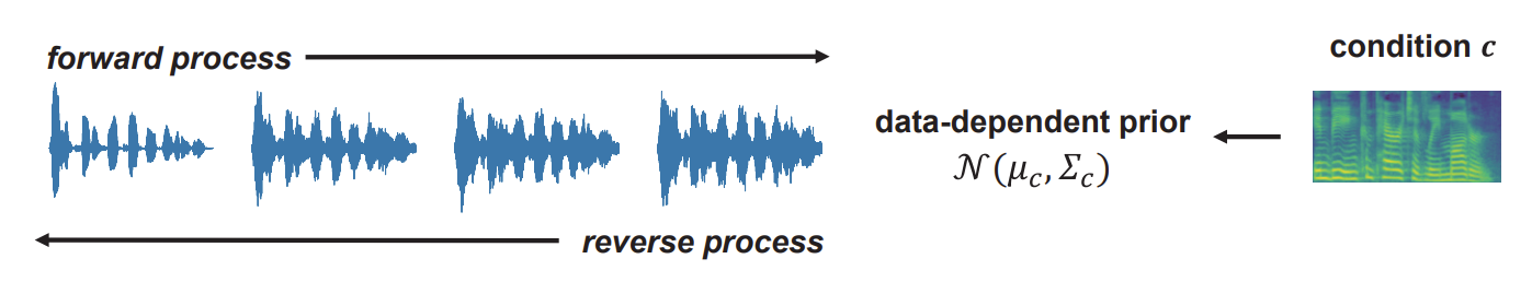
< Overall of PriorGrad >

• Forward diffusion process prior에 대해 non-standard Gaussian 분포를 채택
• Conditional information을 adaptive prior로 활용하여 더 빠른 수렴과 합성 성능을 향상
• 결과적으로 spectral, waveform domain 모두에서 가속화된 추론과 개선된 품질을 달성

2. Background

- Basic Formulation

• DDPM은 2개의 Markov chain (forward / reverse process)으로 구성되는 generative model
  1. Forward process는
     • data $x_{0}$를 standard Gaussian $x_{T}$로 점진적으로 변환:
       (Eq. 1) $q(x_{1:T}|x_{0}) = \prod_{t=1}^{T} q(x_{t}|x_{t-1}), q(x_{t}|x_{t-1}) := \mathcal {N}(x_{t}; \sqrt{1-\beta_{t}}x_{t-1}, \beta_{t}I)$ 
       - $q(x_{t}|x_{t-1})$ : user-defined noise schedule $\beta_{t} \in \{ \beta_{1}, ..., \beta_{T} \}$의 $t$-th step에서의 transition probability
       
     • Noisy 분포 $x_{t}$는 $q(x_{t}|x_{0}) = \mathcal{N}(x_{t};\sqrt{\bar{\alpha}_{t}} x_{0}, (1-\bar{\alpha}_{t})I)$의 closed form
       - 이때 $\alpha_{t} := 1-\beta_{t}$이고, $\bar{\alpha}_{t} := \prod_{s=1}^{t}\alpha_{s}\cdot q(x_{t}|x_{0})$는 noise schedule에 따라 $\bar{\alpha}_{t}$가 충분히 작을 경우 standard Gaussian $\mathcal{N}(x_{T};0,1)$로 수렴
  2. Reverse process는
     • Prior noise를 점진적으로 data로 변환하는 과정으로:
       (Eq. 2) $p_{\theta}(x_{0:T}) = p(x_{T})\prod_{t=1}^{T}p_{\theta}(x_{t-1}|x_{t}), p_{\theta}(x_{t-1}|x_{t}) = \mathcal{N}(x_{t-1};\mu_{\theta}(x_{t},t),\Sigma_{\theta}(x_{t},t))$
       - $p(x_{T}) = \mathcal{N}(x_{T};0,I)$와 $p_{\theta}(x_{t-1}|x_{t})$는 neural network를 통해 parameterize 된 forward transition probability의 역
     • 이때 Evidence Lower BOund (ELBO) loss를 reverse process의 objective로 정의할 수 있음:
       (Eq. 3) $L(\theta) = \mathbb{E}\left[ KL(q(x_{T}|x_{0})||p(x_{T})) + \sum_{t=2}^{T}KL(q(x_{t-1}|x_{t},x_{0})||p_{\theta}(x_{t-1}|x_{t})) - \log p_{\theta}(x_{0}|x_{1})\right]$
     • 여기서 $q(x_{t-1}|x_{t},x_{0})$는 Bayes rule에 따라 아래와 같이 표현됨:
       (Eq. 4) $q(x_{t-1}|x_{t},x_{0}) = \mathcal{N}(x_{t-1};\tilde{\mu}(x_{t},x_{0}), \tilde{\beta}_{t}I)$
       (Eq. 5) $\tilde{\mu}_{t}(x_{t},x_{0}) := \frac{\sqrt{\bar{\alpha}_{t-1}}\beta_{t}}{1-\bar{\alpha}_{t}}x_{0} + \frac{\sqrt{\alpha_{t}}(1-\bar{\alpha}_{t-1})}{1-\bar{\alpha}_{t}}x_{t}, \bar{\beta}_{t} := \frac{1-\bar{\alpha}_{t-1}}{1-\bar{\alpha}_{t}}\beta_{t}$
       
     • $p(x_{T})$를 standard Gaussian으로 고정하면 $KL(q(x_{T}|x_{0})||p(x_{T}))$는 constant가 되므로 parmeterize 될 수 없음
       - 따라서 기존의 framework는 $\Sigma_{\theta}(x_{t},t)$를 constant $\tilde{\beta}_{t}I$로 고정하고, $q(x_{t}|x_{0})$에서 $x_{0}=\frac{1}{\sqrt{\bar{\alpha}_{t}}}(x_{t}-\sqrt{1-\bar{\alpha}_{t}}\epsilon)$를 reparameterize 하여 $\tilde{\mu}_{t}$ 대신 standard Gaussian noise $\epsilon$을 optimization target으로 설정
     • 앞선 설정을 기반으로 각 term의 weighting factor를 줄이고 더 높은 sample 품질을 제공하는 simplifed objective를 얻을 수 있음:
       (Eq. 6) $-ELBO = C + \sum_{t=1}^{T}\mathbb{E}_{x_{0},\epsilon}\left[ \frac{\beta^{2}_{t}}{2\sigma^{2}\alpha_{t}(1-\bar{\alpha}_{t})} || \epsilon - \epsilon_{\theta}(\sqrt{\bar{\alpha}_{t}}x_{0} + \sqrt{1-\bar{\alpha}_{t}}\epsilon, t)||^{2}\right]$
       (Eq. 7) $L_{simple}(\theta):= \mathbb{E}_{t,x_{0},\epsilon}\left[ || \epsilon - \epsilon_{\theta}(x_{t},t)||^{2}\right]$

PriorGrad의 동작 개요

3. Method

• PriorGrad는 infromative prior noise를 data 분포에 가깝게 구성하여 diffusion model의 효율성을 향상하는 것을 목표로 함
  - 이를 위해 non-standard Gaussian을 prior로 사용하여 diffusion model에 대한 일반화된 approach를 제시

Non-Standard Gaussian에서의 Diffusion Trajectory

- General Formulation

• Forward diffusion prior로써 non-standard Gaussian $\mathcal{N}(\mu, \Sigma)$를 사용하기 위해 일반적인 formulation을 유도
  • PriorGrad는 conditional data를 활용하여 adaptive 방식으로 instance level의 근사 prior를 직접 계산하고 학습/추론에 대한 forward diffusion target으로써 해당 근사 prior를 활용
  • 이를 위해 기존 DDPM와 동일하게 $\mu_{\theta}, \sigma_{\theta}$에 대한 parameterization을 활용:
    (Eq. 8) $\mu_{\theta}(x_{t},t)=\frac{1}{\sqrt{\alpha}_{t}}\left( x_{t}-\frac{\beta_{t}}{\sqrt{1-\bar{\alpha}_{t}}}\epsilon_{\theta}(x_{t},t)\right), \sigma_{\theta}(x_{t},t)=\tilde{\beta}^{\frac{1}{2}}_{t}$
  • Forward diffusion prior 분포를 통해 optimal Gaussian $\mathcal{N}(\mu, \Sigma)$에 접근할 수 있다고 가정하면, 다음과 같은 ELBO를 얻을 수 있음:
    [Proposition 1]
    $\epsilon \sim \mathcal{N}(0, \Sigma)$이고 $x_{0} \sim q_{data}$라고 하자. 그러면 (Eq. 8)에 의해 parameterization 되는 ELBO loss는
    $-ELBO = C(\Sigma) + \sum_{t=1}^{T}\gamma \mathbb{E}_{x_{0},\epsilon}|| \epsilon - \epsilon_{\theta}(\sqrt{\bar{\alpha}_{t}}(x_{0}-\mu)+ \sqrt{1-\bar{\alpha}_{t}}\epsilon,t)||_{\Sigma^{-1}}^{2}$
    이때 $C$는 constant이고, $||x||_{\Sigma^{-1}}^{2} = x^{T}\Sigma^{-1}x, \gamma_{t}= \frac{\beta^{2}}{2\sigma^{2}\alpha_{t}(1-\bar{\alpha}_{t})}$는 $t>1$일 때 $\gamma_{1} = \frac{1}{2\alpha_{1}}$이다.

• [Proposition 1]은 non-standard Gaussian 분포를 사용하여 (Eq. 6)을 확장한 것과 동일함
  • Data에 대한 가정 없이 $\mathcal{N}(0,I)$를 사용했던 기존의 DDPM과는 달리 PriorGrad는 [Proposition 1]을 통해 $\mathcal{N}(\mu, \Sigma)$를 사용하여 model을 학습함
    - 이때 각 평균과 분산은 data로부터 추출되어 forward process의 prior로 사용됨
  • 추가적으로 simplified loss $\mathcal{L} = || \epsilon - \epsilon_{\theta}(x_{t}, c,t)||^{2}_{\Sigma^{-1}}$를 위해 $\gamma_{t}$를 제외함
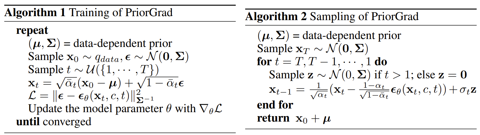
    - 결과적으로 PriorGrad는 data-dependent prior $(\mu, \Sigma)$와 아래의 [Algorithm 1]과 [Algorithm 2]에 의해 학습되고 sampling 됨
    

PriorGrad의 Training, Sampling Algorithm

- Theoretical Analysis

• PriorGrad가 가진 이론적 이점을 분석해 보기 위해,
  • 다음의 simplified modeling을 고려:
    [Proposition 2]
    $L(\mu, \Sigma, x_{0}; \theta)$가 [Proposition 1]의 $-ELBO$ loss를 나타낸다고 하자. 이때 $\epsilon_{\theta}$가 linear function이라고 가정하면, $\det (\Sigma) = \det (I)$ 제약조건 하에서 $\min_{\theta} L(\mu, \Sigma, x_{0}; \theta) \leq \min_{\theta} L(0, I, x_{0};\theta)$이다.
  • [Proposition 2]는 공분산 $\Sigma$과 data $x_{0}$의 공분산을 align 하는 prior 설정하에서 $\epsilon_{\theta}$에 대해 linear function approximation을 사용하는 경우, 더 작은 loss를 얻을 수 있다는 것을 의미
  • 따라서 data-dependent prior 하에서 $q(x_{t-1}|x_{t})$의 평균을 나타내기 위해서는 간단한 model을 사용할 수 있지만, isotropic covariaince가 있는 prior 하에서는 더 복잡한 model을 필요로 한다는 것을 나타냄
    - 이때 condition $\det(\Sigma) = \det (I)$는 두 Gaussian prior가 동일한 entropy를 가진다는 것을 의미
• 다음으로 convergence rate에 대해 이론적 분석을 수행해 보면,
  
  • 최적화에 대한 convergence rate는 loss function의 Hessian matrix $\mathbf{H}$의 condition number에 따라 달라짐
    - 이는 $\frac{\lambda_{\max}(\mathbf{H})} {\lambda_{\min}(\mathbf{H})}$로 나타낼 수 있고, 이때 $\lambda_{\max}, \lambda_{\min}$은 각각 $\mathbf{H}$의 최대, 최소 eigenvalue를 의미
    - Condition 수가 적을수록 convergence rate는 빨라짐
  • $L(\mu, \Sigma, x_{0}; \theta)$에 대해 Hessian은:
    (Eq. 9) $\mathbf{H} = \frac{\partial^{2}L}{\partial \epsilon_{\theta}^{2}} \cdot \frac{\partial \epsilon_{\theta}}{\partial \theta} \cdot \left( \frac{\partial \epsilon_{\theta}}{\partial \theta} \right)^{T} + \frac{\partial L}{\partial \epsilon_{\theta}} \cdot \frac{\partial^{2}\epsilon_{\theta}}{\partial \theta^{2}}$
  • 이때 $\epsilon_{\theta}$가 linear function이라고 가정하면, $L(\mu, \Sigma, x_{0};\theta)$에 대해 $\mathbf{H} \propto I$이고 $L(0,I,x_{0};\theta)$에 대해 $\mathbf{H} \propto \Sigma$
    - 따라서 prior를 $\mathcal{N}(\mu, \Sigma)$로 설정하면 $\mathbf{H}$의 condition 수가 1이 되므로, 가장 작은 condition 수를 얻어 수렴을 가속화할 수 있음

4. Application to Vocoder

- PriorGrad for Vocoder

• PriorGrad Vocoder는 DiffWave를 기반으로 함
  • 이때 model은 data의 compact frequency feature representation을 포함하는 mel-spectrogram에 따라 condition 되어 time-domain waveform을 합성함
    - $\epsilon \sim \mathcal{N}(0,I)$를 사용한 DiffWave와 달리 PriorGrad는 destroyed signal $\sqrt{\bar{\alpha}_{t}}x_{0} + \sqrt{ 1-\bar{\alpha}_{t}}\epsilon$에 대해 noise $\epsilon \sim \mathcal{N}(0, \Sigma)$를 추정하도록 학습됨
  • Network는 diffusion step embedding layer로 얻어지는 noise level의 discreted index $\sqrt{\bar{\alpha}_{t}}$와 conditional projection layer의 mel-spectrogram $c$으로 condition 됨

• Mel-spectrogram condition을 기반으로 data-dependent prior를 얻기 위해
  • Spectral energy가 waveform 분산에 대해 exact correlation을 포함한다는 사실을 기반으로 mel-spectrogram의 normalized frame-level energy를 사용
    1. 먼저 training dataset의 mel-spectrogram $c$에 대한 frame-level energy를 계산하고,
    2. Frame-level energy를 $(0,1]$ 범위로 normalize 하여 data-dependent diagonal variance $\Sigma_{c}$를 얻음
    3. 위를 통해 얻어진 frame-level energy를 waveform에 대한 표준편차의 proxy로 사용
       - 결과적으로 mel-scale spectral energy와 diagonal Gaussian 표준편차 사이의 non-linear mapping이 가능
       
  • PriorGrad는 각 training step에 대한 forward diffusion prior로 $\mathcal{N}(0, \Sigma)$를 설정하고, vocoder의 hop length로 frame-level $\Sigma_{c}$를 waveform-level $\Sigma$로 upsampling
    - 이때 numerical stability를 위해 clipping을 통해 최소 0.1의 표준편차를 가지도록 함

PriorGrad Vocoder의 개요

- Settings

• Dataset : LJSpeech
• Comparisons : DiffWave

- Results

• Model Convergence
  • DiffWave와 PriorGrad의 수렴 속도를 비교해 보면, PriorGrad가 더 빠르게 수렴하는 것으로 나타남
  • PriorGrad는 adaptive prior로 인해 white noise를 쉽게 제거할 수 있지만 DiffWave는 $\epsilon \sim \mathcal{N}(0,I)$에서 시작하므로 reverse process의 denoising 과정이 어렵기 때문

Vocoder 작업에서 수렴 속도 비교

• MOS 측면에서의 합성 품질을 비교해 보면, PriorGrad가 2배 더 적은 학습 iteration만으로도 DiffWave 보다 뛰어난 성능을 보이는 것으로 나타남

MOS 측면에서의 합성 품질 비교 결과

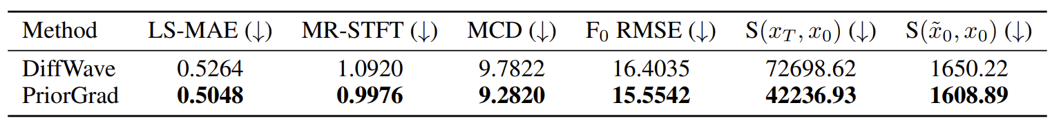
• MR-STFT, MCD와 같은 정량적인 지표 측면에서도 PriorGrad는 더 우수한 성능을 보임

정량적 품질 평가 결과

• Parameter Efficiency
  • Dilated convolution layer의 width를 절반으로 줄여 1.23M의 parameter 수를 가진 smaller model을 구성함
  • 이렇게 얻어진 smaller model에 대해 PriorGrad는 DiffWave보다 더 적은 성능 저하를 보임
    - 결과적으로 smaller PriorGrad를 사용하더라도 기존 model에 가까운 품질을 유지할 수 있고, diffusion model의 parameter efficiency를 향상 가능

Smaller model에 대한 합성 품질 비교

5. Application to Acoustic Model

- PriorGrad for Acoustic Model

• Acoustic model은 encoder-decoder architecture를 사용하여 phoneme sequence에 대한 mel-spectrogram을 생성
  • Acoustic model은 target image가 2D mel-spectrogram인 text-conditional image generation으로 볼 수 있음
    - 이에 대한 성능을 확인하기 위해 PriorGrad를 acoustic model로 확장하여 비교 실험을 수행
  • Adaptive prior를 구축하기 위해 training data에서 동일한 phoneme에 해당하는 frame을 aggregate 하여 80-band mel-spectrogram frame의 phoneme-level statistics를 계산
    - 이때 phoneme-to-frame alignment는 Montreal Forced Alignment (MFA)를 활용
    - 결과적으로 각 phoneme에 대해 training set의 모든 항목을 aggregate 하여 80-dimensional diagonal 평균, 분산을 얻은 다음, phoneme별 $\mathcal{N}(\mu, \Sigma)$ dictionary를 구축
  • Forward diffusion prior에 위의 statistic를 사용하려면, phoneme-level prior sequence를 matching duration을 사용하여 frame-level로 upsampling 해야 함
    - 이를 위해 duration predictor를 활용할 수 있음
    
• [Algorithm 1]을 따라 mean-shifted noisy mel-spectrogram $x_{t}=\sqrt{\bar{\alpha}_{t}}(x_{0}-\mu)+\sqrt{1-\bar{\alpha}_{t}}\epsilon$을 input으로 사용하여 diffusion decoder를 학습함
  • 이때 network는 injected noise $\epsilon \sim \mathcal{N}(0, \Sigma)$를 target으로 추정됨
  • 추가적으로 network는  aligned phoneme encoder output으로 condition 됨
    - Encoder output은 layer-wise $1\times 1$ convolution을 사용하여 gated residual block의 dilated convolution layer의 bias term으로 추가됨

PriorGrad acoustic model의 개요

- Settings

• Dataset : LJSpeech
• Comparisons : FastSpeech2

- Results

• Model Convergence
  • Vocoder와 마찬가지로 acoustic model에서도 PriorGrad를 통해 $\mathcal{N}(\mu, \Sigma)$를 활용하면 수렴 속도가 크게 가속화되고 더 높은 품질의 음성 합성이 가능
  • PriorGrad는 phoneme-level informative forward prior을 통해 diffusion process의 부담을 완화함으로써 학습 초기 단계에서도 고품질 sample 생성이 가능

• Parameter Efficiency
  • Diffusion decoder를 10M에서 3.5M으로 줄였을 때 성능을 비교해 보면, smaller PriorGrad는 기존의 PriorGrad와 거의 동일한 합성 품질을 달성함
  • 결과적으로 PriorGrad는 parameter efficienct 하고 network capacity 감소에도 tolerance 함

Acoustic Model 작업에 대한 성능 비교