[Paper 리뷰] ItoWave: Ito Stochastic Differential Equation is All You Need for Wave Generation

ItoWave: Ito Stochastic Differential Equation is All You Need for Wave Generation

---

• Forward/reverse-time linear stochastic differential equation의 pair에 기반한 vocoder를 구성할 수 있음
• ItoWave
  • Waveform을 tractable distribution으로 변환하는 process와 해당 tractable signal을 target wave로 변환하는 두 가지의 stochastic process를 활용
  • Original mel-spectrogram의 conditional input 하에서 meaningful audio를 생성하기 위해 noise signal에서 excess signal을 점진적으로 제거하는 Wiener process를 활용
• 논문 (ICASSP 20222) : Paper Link

---

1. Introduction

• Neural vocoder는 크게 autoregressive (AR)과 non-autoregressive (non-AR) model로 나눌 수 있음
  • AR model은 previous signal에 따라 current signal frame을 frame-by-frame으로 생성하고, non-AR model은 previous signal에 대한 의존 없이 parallel 하게 생성이 가능함
    1. 일반적으로 AR model은 합성 품질을 보이지만, computation 속도가 상당히 느림
    2. 반면 MelGAN, Parallel WaveGAN 등과 같은 non-AR model은 빠른 합성 속도를 달성할 수 있음
  • 한편으로 linear Ito Stochastic Differential Equation (SDE)를 활용하여 non-AR vocoder를 모델링할 수도 있음
    - 특히 Wiener process에 의해 drive 되는 linear Ito SDE는 waveform data distribution을 white noise와 같은 tractable distribution으로 점진적으로 변환함
  • 결과적으로 대응하는 reverse-time linear Ito SDE를 통해 tractable distribution으로부터 vocoder에 필요한 waveform distribution을 생성할 수 있음
    1. 이때 reverse-time linear SDE의 explicit form은 forward-time equation의 stochastic process solution의 probability density function에 대한 log-value의 gradient에 의존함
       - 여기서 해당 gradient value를 Stein score라고 함
    2. 즉, trained neural network를 통해 waveform에 해당하는 Stein score를 예측한 다음, reverse-time linear Ito SDE나 Langevin dynamic sampling으로 mel-spectrogram과 waveform을 생성할 수 있음

-> 그래서 linear Ito SDE와 score matching modeling을 기반으로 한 ItoWave를 제안

 

• ItoWave
  • Linear Ito SDE를 기반으로 한 neural vocoder를 구성하고 linear SDE의 다양한 drift 및 diffusion coefficent를 selecting
  • Waveform data distribution의 density function에 대한 log-value의 gradient를 효과적으로 추정할 수 있는 network structure를 설계 

< Overall of ItoWave >

• Linear Ito SDE를 기반으로 forward/reverse stochastic process를 통해 waveform을 생성하는 neural vocoder
• 결과적으로 기존 방식들보다 뛰어난 합성 품질을 달성

2. Method

- Audio Data Distribution Transformation based on Ito SDE

• Ito SDE는 다양한 data distribution 간의 transformation을 수행할 수 있음
  • 이때 일반적인 Ito SDE는 $0\leq t\leq T$에서:
    (Eq. 1) $\left\{\begin{matrix}
    d\mathbf{x} =\mathbf{f}(\mathbf{X},t)dt+g(t)d\mathbf{W} \\
    \mathbf{X}(0)=\mathbf{x}(0)
    \end{matrix}\right.$
    - $\mathbf{f}(\cdot, t)$ : drift coefficient, $g(t)$ : diffusion coefficent, $\mathbf{W}$ : standard Wiener process
    
  • $p(\mathbf{x}(t))$를 random variable $\mathbf{X}(t)$의 density라고 하자
    1. 그러면 (Eq. 1)은 Wiener process $\mathbf{W}$로부터 noise를 점진적으로 추가하여 initial distribution $p(\mathbf{x}(0))$을 다른 distribution $p(\mathbf{x}(T))$로 변환함
       - $\mathbf{x}(t)\in\mathbb{R}^{d}$이고, $p(\mathbf{x}(0))$ : ItoWave에서 waveform의 data distribution
       - $p(\mathbf{x}(T))$ : conditional text에 해당하는 mel-spectrogram/latent representation에 대한 Gaussian과 같은 tractable distribution
    2. 이때 해당 stochastic process $\mathbf{x}(t)$가 time에 따라 reverse 될 수 있으면, simple latent distribution으로부터 target mel-spectrogram이나 waveform을 생성할 수 있음 
  • 실제로 reverse-time diffusion process는 $0\leq t\leq T$에 대해 다음의 reverse-time Ito SDE의 solution임:
    (Eq. 2) $\left\{\begin{matrix}
    d\mathbf{X}=[\mathbf{f}(\mathbf{X},t)-g(t)^{2}\nabla_{\mathbf{x}}\log p(\mathbf{x}(t))]dt+g(t)d\bar{\mathbf{W}} \\
    \mathbf{X}(T)=\mathbf{x}(T)
    \end{matrix}\right.$
    - $p(\mathbf{x}(t))$ : $\mathbf{X}(t)$의 distribution, $\bar{\mathbf{W}}$ : reverse-time standard Wiener process
    - (Eq. 2)의 solution은 tractable latent distribution $p(\mathbf{x}(T))$로부터 waveform을 생성하는 데 사용됨
  • 결과적으로 (Eq. 2)에서 SDE를 통해 mel-spectrogram이나 waveform을 생성하기 위해서는  score function $\nabla_{\mathbf{x}}\log p(\mathbf{x}(t))\, (0\leq t\leq T)$를 계산해야 함
    

- Score Estimation of Audio Data Distribution

• ItoWave는 neural network $\mathfrak{S}_{\theta}$를 사용하여 score function을 근사하고, $\theta$는 network parameter를 의미
  • 그러면 network $\mathfrak{S}_{\theta}$는 time $t, \mathbf{x}(t)$, conditional input mel-spectrogram $\mathbf{m}$를 input으로 하여 $\nabla_{\mathbf{x}(t)}\log p(\mathbf{x}(t))$를 output 함 
  • 이때 score matching의 objecitve는:
    (Eq. 3) $\mathbb{E}_{t\sim [0,T]}\mathbb{E}_{\mathbf{x}(t)\sim p(\mathbf{x}(t))}\left[\frac{1}{2} || \mathfrak{S}_{\theta}(\mathbf{x}(t),t,\mathbf{m})-\nabla_{\mathbf{x}(t)}\log p(\mathbf{x}(t)) ||^{2}\right]$
  • 일반적으로 low-density data manifold area에서는 score estimation이 부정확하므로, sampled data의 품질이 저하됨
    1. 만약 mel-spectrogram이나 waveform signal이 small scale noise로 contaminate 되면, 해당 contaminated mel-sepctrogram/signal은 low-dimensional manifold가 아닌 entire space $\mathbb{R}^{d}$로 spread 될 수 있음 
    2. 특히 perturbed mel-spectrogram이나 waveform signal을 input으로 사용하는 경우, 다음의 denoising score matching (DSM) loss가 사용 가능함:
       (Eq. 4) $\textrm{DSM loss} = \mathbb{E}_{t\sim [0,T]}\mathbb{E}_{\mathbf{x}(0)\sim p_{mel}(\mathbf{x}(0))}\mathbb{E}_{\mathbf{x}(t)\sim p(\mathbf{x}(t)|\mathbf{x}(0))}\left[\frac{1}{2}|| \mathfrak{S}_{\theta}(\mathbf{x}(t),t,\mathbf{m})-\nabla_{\mathbf{x}(t)}\log p(\mathbf{x}(t)|\mathbf{x}(0)) ||^{2}\right]$
       - 이는 (Eq. 3)에 대한 Parzen windows density와 같은 non-parametric estimator와 동일함
    3. 결과적으로 해당 DSM loss는 ItoWave의 score prediction network를 training 하는 데 사용됨
       - 여기서 distribution의 score $\nabla_{\mathbf{x}(t)} \log p(\mathbf{x}(t))$를 정확하게 추정할 수 있다면, original distribution에 대한 mel-spectrogram이나 wave sample data를 생성할 수 있음
  • 추가적으로 ItoWave에서는 $\mathcal{L}1$ loss보다 $\mathcal{L}2$ loss를 사용하는 것이 더 효과적임
  • 특히 DSM loss의 transition density $p(\mathbf{x}(t)|\mathbf{x}(0))$와 score $\nabla_{\mathbf{x}(t)}\log p(\mathbf{x}(t)|\mathbf{x}(0))$는 일반적으로 계산하기 어렵지만, linear SDE에 대해 closed formula를 가짐 

- Linear SDE and Transition Densities

• Audio 생성을 위한 linear SDE로써 variance exploding (VE) SDE가 가장 적합함
  • 여기서 VE SDE는:
    (Eq. 5) $\left\{\begin{matrix}
    d\mathbf{X}=\sigma_{0}\left(\frac{\sigma_{1}}{\sigma_{0}}^{t}\sqrt{2\log \frac{\sigma_{1}}{\sigma_{0}}}d\mathbf{W}\right) \\
    \mathbf{X}(0)=\mathbf{x}(0)\sim \int p_{mel}(\mathbf{x})\mathcal{N}(\mathbf{x}(0);\mathbf{x},\sigma_{0}^{2}I)d\mathbf{x}
    \end{matrix}\right.$
    - $\sigma_{0}=0.01 <\sigma_{1}$ 
  • 그러면 transition density $p(\mathbf{x}(t)|\mathbf{x}(0))$의 평균, 분산으로 satisfy 되는 differential equation은:
    (Eq. 6) $\left\{\begin{matrix}
    \frac{d\mathbf{m}(t)}{dt}=0 \\
    \frac{d\mathbf{V}(t)}{dt}=2\sigma_{0}^{2}\left(\frac{\sigma_{1}}{\sigma_{0}}\right)^{2t}\log \frac{\sigma_{1}}{\sigma_{0}}I
    \end{matrix}\right.$
    
  • (Eq. 6)을 solve 하고 $\sigma_{1}$을 choice 하면 $2\log \frac{\sigma_{1}}{\sigma_{0}}=1$이 되고, transition density를 다음과 같이 얻을 수 있음:
    (Eq. 7) $p(\mathbf{x}(t)|\mathbf{x}(0))=\mathcal{N}\left(\mathbf{x}(t);\mathbf{x}(0),\left[\sigma_{0}^{2}\left(\frac{\sigma_{1}}{\sigma_{0}}\right)^{2t}-\sigma_{0}^{2} \right]I\right)$
  • 그러면 VE linear SDE의 score는:
    (Eq. 8) $\nabla_{\mathbf{x}(t)}\log p(\mathbf{x}(t)|\mathbf{x}(0))=\nabla_{\mathbf{x}(t)}\log \mathcal{N}\left(\mathbf{x}(t);\mathbf{x}(0),\left[\sigma_{0}^{2}\left(\frac{\sigma_{1}}{\sigma_{2}}\right)^{2t}-\sigma_{0}^{2}\right]I\right)$
    $\,\,\,\,\,\,\,\,\,\,\,\,\,\,\,\,\,\,\,=\nabla_{\mathbf{x}(t)}\left[-\frac{d}{2}\log \left[ 2\pi\left(\sigma_{0}^{2}\left(\frac{\sigma_{1}}{\sigma_{0}}\right)^{2t}-\sigma_{0}^{2}\right)\right]-\frac{|| \mathbf{x}(t)-\mathbf{x}(0)||^{2}}{2\left(\sigma_{0}^{2}\left(\frac{\sigma_{1}}{\sigma_{0}}\right)^{2t}-\sigma_{0}^{2}\right)}\right] = -\frac{\mathbf{x}(t)-\mathbf{x}(0)}{\sigma_{0}^{2}\left(\frac{\sigma_{1}}{\sigma_{2}}\right)^{2t}-\sigma_{0}^{2}}$
  • Piror distribution $p(\mathbf{x}(T))$는 Gaussian이 됨:
    (Eq. 9) $\mathcal{N}(\mathbf{x}(T);0,\sigma_{1}^{2}I)=\frac{\exp \left( -\frac{1}{2\sigma_{1}^{2}}|| \mathbf{x}(T)||^{2}\right)}{\sigma_{1}^{d}\sqrt{(2\pi)^{d}}}$
    - 따라서 $\log p(\mathbf{x}(T))=-\frac{d}{2}\log(2\pi\sigma_{1}^{2})-\frac{1}{2\sigma_{1}^{2}}|| \mathbf{x}(T) ||^{2}$

Training Algorithm

- Training and Wave Sampling Algorithms

• 앞선 formulation들을 기반으로 위의 [Algorithm 1]과 같이 general SDE를 기반으로 한 score matching network training이 가능함
  • 먼저 loss minimization을 통해 optimal score network $\mathfrak{S}_{\theta_{*}}$을 얻은 다음, $\mathfrak{S}_{\theta_{*}}(\mathbf{x}(t),t,\mathbf{m})$을 사용하여 waveform distribution의 probability density에 대한 log-value의 gradient를 얻을 수 있음
    1. 이후 Langevin dynamics나 (Eq. 2)의 reverse-time Ito SDE를 사용하여 specific mel-spectrogram $\mathbf{m}$에 해당하는 waveform을 생성함
    2. 이때 time schedule이 fix 되어 있다고 가정하면, (Eq. 1)의 diffusion process에 대한 discretization은:
       (Eq. 10) $\left\{\begin{matrix}
       \mathbf{X}(i\Delta t+\Delta t)-\mathbf{X}(i\Delta t) =\mathbf{f}(\mathbf{X}(i\Delta t),i\Delta t)\Delta t + g(i\Delta t)\xi (i\Delta t), (i=0,1,...,N-1)\\
       \mathbf{X}(0)=\mathbf{x}(0)
       \end{matrix}\right.$
       - $d\mathbf{W}$는 wide sense stationary white noise process이므로, $\xi(\cdot)\sim \mathcal{N}(0,I)$로 나타낼 수 있음
    3. 그러면 (Eq. 2)의 reverse-time diffusion process에 대한 discretization은:
       (Eq. 11) $\left\{\begin{matrix}
       \mathbf{X}(i\Delta t)-\mathbf{X}(i\Delta t+\Delta t)\\
       =\mathbf{f}(\mathbf{X}(i\Delta t+\Delta t),i\Delta t+\Delta t)(-\Delta t)-g(i\Delta t+\Delta t)^{2}\mathfrak{S}_{\theta_{*}}(\mathbf{X}(i\Delta t+\Delta t),i\Delta t+\Delta t, \mathbf{m})(-\Delta t) \\
       \mathbf{X}(T)=\mathbf{x}(T)
       \end{matrix}\right.$
       - $T=N\Delta t, i=0,1,...,N-1$
  • 논문에서는 SDE Score Matching과 같이 각 time step에서 Langevin dynamics를 사용하여 예측을 수행한 다음, (Eq. 11)의 reverse-time Ito SDE를 통해 first prediction result를 revise 함
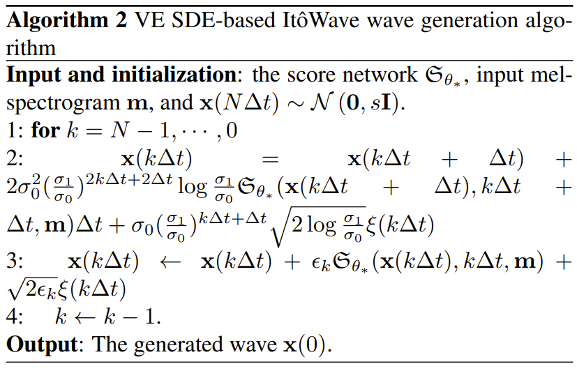
    - 이때 VE linear SDE를 통한 generation은 아래 [Algorithm 2]와 같이 수행됨

Waveform Generation Algorithm

- Architectures of $\mathfrak{S}_{\theta}(\mathbf{x}_{t},t,\mathbf{m})$

• Score network model은 flow model 만큼의 strict restriction을 가지지는 않지만, 모든 network structure가 score prediction에 적합한 것은 아님
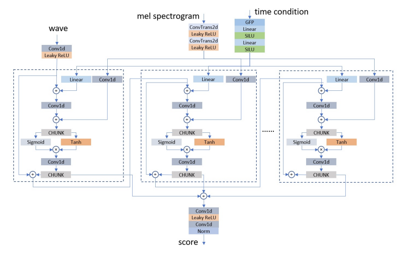
  • 따라서 ItoWave는 score network $\mathfrak{S}_{\theta}(\mathbf{x}(t),t,\mathbf{m})$으로써 아래 그림과 같은 structure를 활용하여 time $t$에서의 score를 output 함
  • 먼저 waveform은 convolution layer를 통해 preprocess 되고, mel-spectrogram은 2개의 transposed convolution layer를 통한 upsampling layer로 처리됨
    1. 해당 input들이 preprocess 되면 serially connected dilated residual block으로 전달됨
       - Dilated residual block은 wave를 main input으로 사용하고, time condition과 mel-spectrogram condition은 해당 dilated residual block에 차례로 input 된 다음, wave signal transformation이후 feature map에 추가됨
    2. 이때 각 dilated residual block은 다음 residual block의 input으로 사용되는 state와 final output에 대한 2개의 output을 가짐
       - 이를 통해 다양한 granularity의 information을 반영할 수 있음
    3. 최종적으로 모든 residual block의 output을 summation 한 다음, final output score를 얻기 위해 2개의 convolution layer를 적용함

ItoWave Architecture

3. Experiments

- Settings

• Dataset : LJSpeech 
• Comparisons : WaveNet, WaveGlow, DiffWave, WaveGrad

- Results

• MOS 측면에서 ItoWave는 가장 뛰어난 성능을 달성함

모델 성능 비교

• 아래 그림과 같이 ItoWave는 매 step 마다 Gaussian noise를 점진적으로 개선하는 것을 확인할 수 있음 

Step 별 Frequency Spectrum 비교