[Paper 리뷰] BDDM: Bilateral Denoising Diffusion Models for Fast and High-Quality Speech Synthesis

BDDM: Bilateral Denoising Diffusion Models for Fast and High-Quality Speech Synthesis

---

• Diffusion model은 우수한 합성 품질을 보이고 있지만 효율적인 sampling의 어려움이 있음
• Bilateral Denoising Diffusion Model (BDDM)
  • Bilateral modeling objective로 train 할 수 있는 schedule network와 score network를 사용하여 forward/reverse process를 parameterize 하는 bilateral denoising diffusion model
  • 제안된 surrogate objective는 기존 surrogate보다 tighter 한 log marginal likelihood의 lower bound를 달성할 수 있음
  • BDDM은 모든 pre-trained score network parameter를 inheriting 할 수 있으므로, schedule network를 빠르고 안정적으로 최적화할 수 있음
• 논문 (ICLR 2022) : Paper Link

---

1. Introduction

• Vocoder는 주로 Generative Adversarial Network (GAN)-based와 likelihood-based 방식을 주로 활용함
  • GAN-based 방식은 adversarial training을 활용하므로 training 과정이 unstable 할 수 있음
  • Likelihood-based 방식은 training을 위해 log-likelihood나 surrogate objective를 사용하지만 생성 속도의 한계가 있음
    - 대표적으로 autoregressive model은 high-fidelity의 음성을 합성할 수 있지만, 상당히 느린 sampling process를 보임
    - VAE의 lower bound나 contrastive divergence 같은 surrogate objective는 합성 속도는 향상할 수 있지만, 일반적으로 GAN-based 방식보다 낮은 품질을 보임
  • 한편으로 likelihood-based model로써 최근의 Diffusion Probabilistic Model (DPM)을 고려할 수 있음
    1. Forward diffusion process를 사용하여 주어진 분포를 sequentially corrupt 하고, reverse process를 통해 data 분포를 restore 하는 방식
    2. 이때 score matching을 활용하는 score-based generative model을 통해 Langevin dynamics로 sampling 하는 neural network를 training 할 수 있음
       - 대표적으로 Denoising Diffusion Probabilistic Model (DDPM)은 해당 방식을 사용하여 GAN-based model 보다 뛰어난 성능을 달성
       - 음성 합성 측면에서도 WaveGrad, DiffWave 같은 모델들이 DDPM을 활용하여 우수한 성능을 달성함
  • BUT, 여전히 vocoder 작업에서 diffusion model은 GAN에 비해 느린 합성 속도를 보임
    - Target distribution을 학습하기 위해 training 중에 수천번의 diffusion step이 필요하기 때문
    - 이때 sampling step을 줄이기 위해 noise scheduling과 같은 방식을 도입할 수 있음

-> 그래서 vocoder 작업에서 diffusion model의 합성 속도를 개선하는 BDDM을 제안

 

• BDDM
  • Schedule network와 score network를 사용하여 forward/reverse process를 parameterize 함
    - 이때 score network가 최적화된 다음에 schedule network가 training 되어야 함
  • 따라서 schedule network의 training을 위해 새로 유도된 lower bound와 log marginal likelihood 간의 gap을 최소화하는 objective를 설계
  • 추가적으로 빠르고 고품질의 합성을 위한 sampling algorithm을 제시

< Overall of BDDM >

• Bilateral modeling objective로 train 할 수 있는 schedule network와 score network를 사용하여 forward/reverse process를 parameterize
• 기존 surrogate objective보다 tighter 한 log marginal likelihood의 lower bound를 달성하고, 모든 pre-trained score network parameter를 inheriting 하여 schedule network를 빠르고 안정적으로 최적화함
• 결과적으로 diffusion model의 우수한 합성 품질을 유지하면서 기존보다 최대 143배 빠른 합성 속도를 달성 

2. Background

- Diffusion Probabilistic Model (DPM)

• Unknown data distribution $p_{data}(x_{0})$의 $i.i.d.$ sample $\{x_{0}\in \mathbb{R}^{D}\}$가 주어지면,
  • Diffusion Probabilistic Model (DPM)은 $T$ step의 diffusion을 통해 complex data distribution을 tractable distribution으로 변환하는 forward process $q(x_{1:T}|x_{0})=\prod_{t=1}^{T}q(x_{t}|x_{t-1})$를 정의함
  • $\theta$로 parameterize 된 reverse process $p_{\theta}(x_{t-1}|x_{t})$는 data distribution을 모델링하는 데 사용됨:
    $p_{\theta}(x_{0})=\int \pi(x_{T})\prod_{t=1}^{T}p_{\theta}(x_{t-1}|x_{t})dx_{1:T}$
    - $\pi(x_{T})$ : reverse process를 시작하기 위한 prior distribution
  • 그러면 standard log Evidence Lowe BOund (ELBO)를 최대화하여 variational parameter $\theta$를 학습할 수 있음:
    (Eq. 1) $\mathcal{F}_{elbo}:=\mathbb{E}_{q}\left[\log p_{\theta}(x_{0}|x_{1})-\sum_{t=2}^{T}D_{KL}(q(x_{t-1}|x_{t},x_{0})||p_{\theta}(x_{t-1}|x_{t}))-D_{KL}(q(x_{T}|x_{0})|| \pi(x_{T}))\right]$

- Denoising Diffusion Probabilistic Model (DDPM)

• 앞선 DPM의 확장으로, DDPM은 score mathcing을 사용하여 reverse process를 정의함
  • 특히 DDPM은 $0<\beta_{1},...,\beta_{T}<1$인 noise schedule $\beta \in \mathbb{R}^{T}$에 의해 parameterize 된 Gaussian diffusion process를 고려함:
    (Eq. 2) $q_{\beta}(x_{1:T}|x_{0}):=\prod_{t=1}^{T}q_{\beta_{t}}(x_{t}|x_{t-1}),\,\,\mathrm{where}\,\, q_{\beta_{t}}(x_{t}|x_{t-1}):=\mathcal{N}(\sqrt{1-\beta_{t}}x_{t-1},\beta_{t}I)$
  • Isotropic Guassian의 property를 기반으로 $x_{0}$에 대해 directly condition 된 $x_{t}$를 나타낼 수 있음:
    (Eq. 3) $q_{\beta}(x_{t}|x_{0})=\mathcal{N}(\alpha_{t}x_{0},(1-\alpha^{2}_{t})I),\,\, \mathrm{where}\,\, \alpha_{t}=\prod_{i=1}^{t}\sqrt{1-\beta_{i}}$
  • 해당 forward process를 revert 하기 위해, DDPM은 score network $\epsilon_{\theta}(x_{t},\alpha_{t})$를 사용해 다음을 정의함:
    (Eq. 4) $p_{\theta}(x_{t-1}|x_{t}):=\mathcal{N}\left(\frac{1}{\sqrt{1-\beta_{t}}}\left(x_{t}-\frac{\beta_{t}}{\sqrt{1-\alpha_{t}^{2}}}\epsilon_{\theta}(x_{t},\alpha_{t})\right),\Sigma_{t}\right)$
    - $\Sigma_{t}$ : reverse process에 대해 정의된 covariance matrix
    - $\Sigma_{t} =\tilde{\beta}_{t}I=\frac{1-\alpha_{t-1}^{2}}{1-\alpha_{t}^{2}}\beta_{t}I$은 deterministic $x_{0}$에 optimal하고, $\Sigma_{t}=\beta_{t}I$는 white noise $x_{0}\sim \mathcal{N}(0,I)$에 optimal함
  • 한편으로 두 optimal을 jointly trained neural network로 interpolate 하는 learnable variance를 고려할 수 있음:
    $\Sigma_{t,\theta}(x):=\mathrm{diag}(\exp(v_{\theta}(x)\log\beta_{t}+(1-v_{\theta}(x))\log\tilde{\beta}_{t}))$
    - $v_{\theta}(x)\in\mathbb{R}^{D}$ : trainable network
  • (Eq. 1)에서 completer ELBO를 계산하려면 score network에 대해 $T$개의 forward pass가 필요하므로 large $T$에 대한 training은 computationally prohibitive 함
    1. 따라서 score network를 training 하기 위해 complete ELBO를 계산하는 대신, discrete uniform distribution $t\sim \mathcal{U}\{1,...,T\}, \, x_{0}\sim p_{data}(x_{0}),\, \epsilon_{t}\sim\mathcal{N}(0,I)$에서 sampling 하여,
    2. 각 training iteration에서 training loss를 계산함:
       (Eq. 5) $\mathcal{L}_{ddpm}^{(t)}(\theta):= \left| \left| \epsilon_{t}-\epsilon_{\theta}\left(\alpha_{t}x_{0}+\sqrt{1-\alpha_{t}^{2}}\epsilon_{t},\alpha_{t}\right) \right| \right|_{2}^{2}$
       - 이는 $D_{KL}(q_{\beta}(x_{t-1}|x_{t},x_{0})||p_{\theta}(x_{t-1}|x_{t}))$의 re-weighting form과 같음
       

3. Bilateral Denoising Diffusion Model (BDDM)

- Problem Formulation

• BDDM은 빠른 sampling을 위해 training noise schedule $\beta$보다 짧은 sampling noise schedule $\hat{\beta}$를 사용함
  • 이를 위해 각각의 noise schedule $\beta, \hat{\beta}$에 해당하는 2개의 개별적인 diffusion process를 정의
    - 여기서 $\beta$에 의해 parameterize 된 upper diffusion process는 (Eq. 2)와 동일하지만, lower process는 더 적은 diffusion step $(N\ll T)$를 가지는 $q_{\hat{\beta}}(\hat{x}_{1:N}| \hat{x}_{0})=\prod_{n=1}^{N}q_{\hat{\beta}_{n}}(\hat{x}_{n}| \hat{x}_{n-1})$로 정의됨
  • 이때 problem formulation 과정에서 $\beta$는 주어지지만, $\hat{\beta}$는 unknown임
  • 따라서 $\hat{x}_{0}$가 $N$개의 reverse step을 통해 $\hat{x}_{N}$에서 효과적으로 recover 될 수 있도록 reverse process $p_{\theta}(\hat{x}_{n-1}| \hat{x}_{n};\hat{\beta}_{n})$에 대한 $\hat{\beta}$를 찾는 것을 목표로 함

- Model Description

• 기존에는 shortened linear나 Fibonacci noise schedule을 reverse process에 사용함
  • 이론적으로, shortened noise schedule로 specify 된 diffusion process는 score network $\theta$를 training 하는 데 사용된 것과 다름
    - 따라서 $\theta$는 shortened diffusion process를 revert 하는데 적합하지 않음
  • 해당 문제를 해결하기 위해 shortened schedule $\hat{\beta}$와 score network $\theta$ 간의 연결을 설정하는 모델링 방식이 필요함 (즉, $\theta$에 따라 $\hat{\beta}$를 최적화해야 함)
  • 먼저 starting point로써 $N=\lfloor T /\tau \rfloor$을 고려하자
    1. 여기서 $1\leq \tau \leq T$는 step size를 control 하는 hyperparameter로써, shorter diffusion process에서 두 consecutive variable 간의 diffusion step은 longer diffusion step의 $\tau$ diffusion step에 해당
    2. 그러면 (Eq. 2)에 따라:
       (Eq. 6) $q_{\hat{\beta}_{n+1}}(\hat{x}_{n+1}| \hat{x}_{n}=x_{t}):=q_{\beta}(x_{t+\tau}|x_{t})=\mathcal{N}\left(\sqrt{\frac{\alpha_{t+\tau}^{2}}{\alpha_{t}^{2}}}x_{t},\left(1-\frac{\alpha_{t+\tau}^{2}}{\alpha_{t}^{2}}\right)I\right)$
       - $x_{t}$ : 2개의 서로 다른 indexed diffusion sequence를 연결하는 intermediate diffused variable
       - 즉, $x_{t}=\alpha_{t}x_{0}+\sqrt{1-\alpha_{t}^{2}}\epsilon_{n}$은 training 중에 $x_{0}, \beta$가 주어지면 쉽게 생성될 수 있는 junctional variable
  • BUT, $x_{0}$가 주어지지 않는 reverse process의 경우 앞선 junctional variable은 intractable 함
    1. 여기서 long $\beta$-parameterized diffusion process로 train 된 score network $\theta^{*}$를 사용할 때, schedule network $\phi$를 도입하여 short noise schedule $\hat{\beta}(\phi)$를 최적화할 수 있음
    2. 결과적으로 BDDM은 score network와 schedule network에 대한 training objective $\mathcal{L}_{score}^{(n)}(\theta)$와 $\mathcal{L}_{step}^{(n)}(\phi;\theta^{*})$을 사용하여 최적화됨

Overall of BDDM

- Score Network

• 먼저 DDPM은 white noise $x_{T}\sim \mathcal{N}(0,I)$를 사용하는 reverse process를 통해 data distribution을 $T$ step에 걸쳐 recover 함:
  (Eq. 7) $p_{\theta}(x_{0}) \overset{DDPM}{:=} \mathbb{E}_{\mathcal{N}(0,I)}\left[\mathbb{E}_{p_{\theta}(x_{1:T-1}|x_{T})}[p_{\theta}(x_{0}|x_{1:T})]\right]$
• 이와 달리 BDDM은,
  • Junctional variable $x_{t}$에서 시작하여 $n$ step만으로 더 짧게 diffusion random variable를 revert 함:
    (Eq. 8) $p_{\theta}(\hat{x}_{0}) \overset{BDDM}{:=}\mathbb{E}_{q_{\hat{\beta}}(\hat{x}_{n-1};x_{t},\epsilon_{n})}\left[\mathbb{E}_{p_{\theta(\hat{x}_{1:n-2}|\hat{x}_{n-1})}}[p_{\theta}(\hat{x}_{0}| \hat{x}_{1:n-1})]\right], \,\, 2\leq n \leq N$
  • 여기서 $q_{\hat{\beta}}(\hat{x}_{n-1};x_{t},\epsilon_{n})$은 posterior에 대한 reparameterization으로 정의됨:
    (Eq. 9) $q_{\hat{\beta}}(\hat{x}_{n-1};x_{t},n) := q_{\hat{\beta}}\left( \hat{x}_{n-1}\left| \hat{x}_{n}=x_{t},\hat{x}_{0}=\frac{x_{t}-\sqrt{1-\hat{\alpha}_{n}^{2}}\epsilon_{n}}{\hat{\alpha}_{n}}\right.\right)$
    (Eq. 10) $\,\,\,\,\,\,\,\,\,\,\,\,\,\,\,\,\,\,\,\,\,\,\,\,\,\,\,\,\,\,\,\,\,\,\,\,= \mathcal{N}\left( \frac{1}{\sqrt{1-\hat{\beta}_{n}}}x-\frac{\hat{\beta}_{n}}{\sqrt{(1-\hat{\beta}_{n})(1-\hat{\alpha}_{n}^{2})}}\epsilon_{n}, \frac{1-\hat{\alpha}_{n-1}^{2}}{1-\hat{\alpha}_{n}^{2}}\hat{\beta}_{n}I \right)$
    - $\hat{\alpha}_{n}=\prod_{i=1}^{n}\sqrt{1-\hat{\beta}_{i}}, \,\, x_{t}=\alpha_{t}x_{0}+\sqrt{1-\alpha_{t}^{2}}\epsilon_{n}$ : approximate index $t\sim \mathcal{U}\{(n-1)\tau, ..., n\tau -1, n\tau\}$와 sampled white noise $\epsilon_{n}\sim \mathcal{N}(0,I)$가 주어지면 $x_{t}$를 $\hat{x}_{n}$에 mapping 하는 junctional variable

- Training Objective for Score Network

• 위의 정의를 사용하면, $\log p_{\theta}(\hat{x}_{0})\geq \mathcal{F}_{score}^{(n)}(\theta):=-\mathcal{L}_{score}^{(n)}(\theta)-\mathcal{R}_{\theta}(\hat{x}_{0},\hat{x}_{t})$와 같은 log marginal likelihood에 대한 새로운 form의 lower bound를 얻을 수 있음
  • 여기서:
    (Eq. 11) $\mathcal{L}_{score}^{(n)}(\theta):=D_{KL}\left(p_{\theta}(\hat{x}_{n-1}| \hat{x}=x_{t})||q_{\hat{\beta}}(\hat{x}_{n-1};x_{t},\epsilon_{n})\right)$
    (Eq. 12) $\mathcal{R}_{\theta}(\hat{x}_{0},x_{t}):=-\mathbb{E}_{p_{\theta}(\hat{x}_{1}|\hat{x}_{n}=x_{t})}[\log p_{\theta}(\hat{x}_{0}| \hat{x}_{1})]$
  • 이때 junctional variable $x_{t}$를 통해 $\theta^{*}$이 $\mathcal{L}_{ddpm}^{(t)}(\theta),\, \forall t\in \{1,...,T\}$를 최적화하기 위한 solution임을 증명할 수 있음
    - 이는 $\mathcal{L}_{score}^{(n)}(\theta),\,\, \forall n \in \{2,...,N\}$을 최적화하는 solution이기도 함
    - 결과적으로 score network $\theta$가 $\mathcal{L}_{ddpm}^{(t)}(\theta)$로 train 될 수 있고, $\hat{x}_{N:0}$에 대한 short diffusion process를 revert하기 위해 reuse될 수 있음
  • 이러한 BDDM의 새로운 lower bound는 기존의 score network와 동일한 objective를 가지지만, score network $\theta$와 $\hat{x}_{N:0}$ 사이의 연결을 설정할 수 있음
    - 해당 연결은 $\hat{\beta}$ 학습에 필수적으로 사용됨

- Schedule Network

• BDDM에서는 schedule network에 $\hat{\beta}_{n}$을 $\hat{\beta}_{n}(\phi)=f_{\phi}\left(x_{t};\hat{\beta}_{n+1}\right)$로 reparameterizing 한 forward process를 도입함
  • 이때 training 중에 $x_{t}=\alpha_{t}x_{0}+\sqrt{1-\alpha_{t}^{2}}\epsilon_{n}, \, \, \hat{\beta}_{n+1}=1-\frac{\alpha^{2}_{t+\tau}}{\alpha_{t}^{2}}$를 사용할 수 있음
  • 해당 reparameterization을 통해 noise scheduling (i.e., $\hat{\beta}$ 탐색)은 data-dependent variance를 ancestrally estimate 하는 schedule network $f_{\phi}$를 training 하는 것으로 reformulate 됨
    - 여기서 schedule network는 current noisy sample $x_{t}$를 기반으로 $\hat{\beta}_{n}$을 예측하는 방법을 학습함
    - Diffusion step information을 반영하는 $\hat{\beta}_{n+1}, t, n$ 외에도 $x_{t}$는 추론 시 reverse direction의 noise scheduling에 필수적인 것으로 나타남
  • 이를 위해 ancestral step information $\hat{\beta}_{n+1}$을 채택해 current step에 대한 upper bound를 도출하고, schedule network는 current noisy sample $x_{t}$를 input으로 사용해 ancestral step에 대한 noise scale의 relative change를 예측함
    1. 따라서 먼저 $0<\hat{\beta}_{n}<\min\left\{ 1-\frac{\hat{\alpha}^{2}_{n+1}}{1-\hat{\beta}_{n+1}},\hat{\beta}_{n+1}\right\}$에 대한 증명을 통해 $\hat{\beta}_{n}$에 대한 upper bound를 유도한 다음,
    2. 그리고 upper bound에 neural network로 추정된 ratio $\sigma_{\phi}:\mathbb{R}^{D}\mapsto (0,1)$를 곱하여 다음을 정의:
       (Eq. 13) $f_{\phi}(x_{t};\hat{\beta}_{n+1}):=\min\left\{ 1-\frac{\hat{\alpha}_{n+1}^{2}}{1-\hat{\beta}_{n+1}},\hat{\beta}_{n+1}\right\}\sigma_{\phi}(x_{t})$
       - 여기서 network parameter set $\phi$는 current noisy input $x_{t}$에서 2개의 consecutive noise scale $\hat{\beta}_{n},\hat{\beta}_{n+1}$ 사이의 ratio를 추정하기 위해 학습됨
  • 최종적으로 추론 시 noise scheduling을 위해, maximum reverse step $N$과 2개의 hyperparameter $\hat{\alpha}_{N}, \hat{\beta}_{N}$에서 시작해
    1. $\hat{\beta}_{n}(\phi)=f_{\phi}\left(\hat{x}_{n};\hat{\beta}_{n+1}\right)$를 $N$에서 1까지의 $n$에 대해 ancestrally predict 하고,
    2. $\hat{\alpha}_{n}=\frac{\hat{\alpha}_{n+1}}{\sqrt{1-\hat{\beta}_{n+1}}}$를 cumulatively update 함

- Training Objective for Schedule Network

• Network parameter $\phi$를 효과적으로 학습하기 위해서는 $\theta$가 well-optimize 된 다음에, $\phi$가 training 되어야 함
  
  • 이는 lower bound $\mathcal{F}_{score}^{(n)}(\theta^{*})$과 $\log p_{\theta^{*}}(\hat{x}_{0})$의 차이, $\log p_{\theta^{*}}(\hat{x}_{0})-\mathcal{F}_{score}^{(n)}(\theta^{*})$을 최소화해야 하는 것을 의미
    
  • 즉, 다음의 objective를 최소화함:
    (Eq. 14) $\mathcal{L}_{step}^{(n)}(\phi;\theta^{*}):=D_{KL}\left( p_{\theta^{*}}(\hat{x}_{n-1}|\hat{x}_{n}=x_{t})|| q_{\hat{\beta}_{n}(\phi)}(\hat{x}_{n-1};x_{0},\alpha_{t})\right)$
    - 이는 $p_{\theta^{*}}(\hat{x}_{n-1}|\hat{x}_{n}=x_{t})$를 reparameterized forward process에 대한 KL divergence로 정의되고, junctional noise scale $\alpha_{t}$와 $x_{0}$로 condition 될 때 tractable 해짐

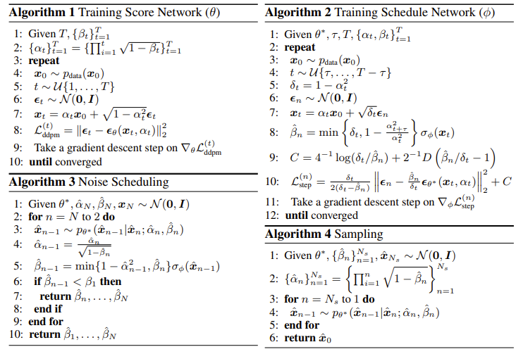
4. Algorithms: Training, Noise Scheduling, and Sampling

- Training Score and Schedule Networks

• $\phi$를 학습하기 전에 $\theta$를 먼저 최적화해야 함
  • 따라서 score network $\epsilon_{\theta}$를 training 하기 위해 $\beta$를 linear noise schedule로 설정함:
    $\beta_{t}=\beta_{start}+\frac{t}{T}(\beta_{end}-\beta_{start})$
    - $1\leq t \leq T$이고, $\beta_{start}, \beta_{end}$ : start, end value를 specify 하는 hyperparameter
    - 결과적으로 training은 아래의 [Algorithm 1]과 같이 동작하게 됨
  • 다음으로 수렴된 score network $\theta^{*}$을 기반으로 schedule network $\phi$를 training 함
    1. 각 training step에서 $n\sim\mathcal{U}\{2,...,N\}$을 draw 한 다음, $t\sim \mathcal{U}\{(n-1)\tau,...,n\tau\}$를 draw 함
       - 이는 fine-scale time step에 대해 $t\sim \mathcal\{\tau,...,T-\tau\}$를 직접 draw 하는 것으로 re-formulate 될 수 있음
    2. 이후 [Algorithm 2]와 같이 $\mathcal{L}_{step}^{(n)}(\phi,\theta^{*})$을 계산하는데 필요한 variable을 sequentially compute 함
       - 여기서 linear schedule이 $\beta$를 정의하는 데 사용되지만, $f_{\phi}$에 의해 예측된 $\hat{\beta}$의 nosie schedule은 linear schedule에 국한되지 않는 것으로 나타남

- Noise Scheduling for Fast and High-Quality Sampling

• Score network와 schedule network가 train 된 이후의 추론 procedure는 2단계로 나눌 수 있음
  1. Noise Scheduling Phase
     • 먼저 $N$의 maximum iteration을 사용하여 sampling process와 유사하게 noise scheduling process를 수행
       - 이때 $\alpha_{t}$가 forward-compute 되는 training 과정과는 달리, 추론에 사용되는 $\hat{\alpha}_{n}$은 noise scheduling phase에서 $\{\hat{\beta}\}^{n-1}_{i}$가 unknown이기 때문에 $N$에서 1로 backward-compute 됨
     • 따라서 noise scheduling을 시작하기 위해 $\hat{\alpha}_{N}$,$\hat{\beta_{N}}$의 두 hyperparameter를 설정
       - 가장 작은 noise scale $\beta_{1}$을 threshold로 사용하여 noise scheduling process를 early stop 하면, score network의 training에서 나타나지 않은 small noise scale ($<\beta_{1}$)을 무시할 수 있음
       - 결과적으로 noise scheduling process는 [Algorithm 3]과 같이 진행됨
  2. Sampling Phase
     • $(\hat{\alpha}_{N}, \hat{\beta}_{N})$에 대한 적절한 값을 찾기 위해, [Algorithm 3]에 대해 $\mathcal{O}(M^{2})$이 소모되는 $M$ bin의 gird search algorithm을 적용함
       - 논문에서는 $M=9$ 사용
     • Noise scheduling algorithm에 대한 grid search는 training sample의 small subset으로 evaluate 될 수 있고, 경험적으로 1개의 sample만 있더라도 BDDM에서는 잘 동작하는 것으로 나타남
     • 최종적으로 예측된 noise scheduel $\hat{\beta}\in \mathbb{R}^{N_{s}}$가 주어지면, [Algorithm 4]와 같이 $N_{s}$ sampling step으로 sample을 생성함

Training, Sampling, Noise Scheduling Algorithm

5. Experiments

- Settings

• Dataset : LJSpeech, VCTK
• Comparisons : WaveNet, WaveGlow, MelGAN, HiFi-GAN, WaveGrad, DiffWave

- Results

• Sampling Quality
  • 7-step, 12-step BDDM이 ground-truth와 가장 비슷한 합성 품질을 달성함
  • 특히 BDDM은 RTF 측면에서 WaveGrad보다 143배 빠르고, DiffWave보다 28.6배 빠름

성능 비교 결과

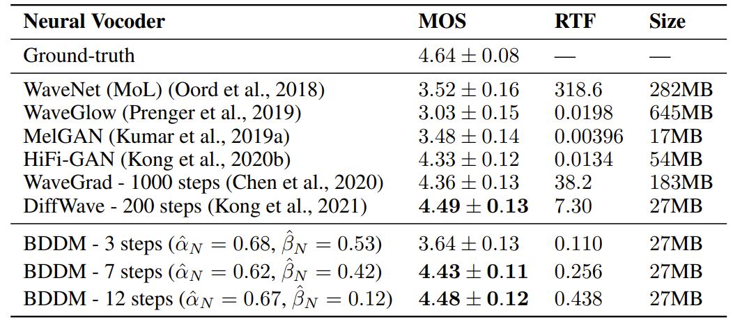
• BDDM과 다른 accelerated sampling을 비교해 보면
  • FS method는 큰 성능 저하가 발생하고, DDIM과 NE method는 모든 step에서 안정적으로 동작하나 충분한 성능을 달성하지 못함
  • 반면 BDDM은 모든 step에 대해 일관적으로 우수한 성능을 보임

Acceleration Method 비교

• Ablation Study and Analysis
  • BDDM의 loss를 standard negative ELBO로 대체해 보면
  • $\mathcal{L}_{elbo}^{(n)}$을 사용할 때 network는 0으로 빠르게 collapse 하는 것으로 나타남
  • 반면 $\mathcal{L}^{(n)}$ step을 사용하면 network는 fluctuating output을 생성함
    - 이러한 fluctuation은 network가 $t$-dependent noise scale을 적절히 예측한다는 것을 의미함
    

Ablation Study 결과