[Paper 리뷰] DFlow: A Generative Model Combining Denoising AutoEncoder and Normalizing Flow for High Fidelity Waveform Generation

DFlow: A Generative Model Combining Denoising AutoEncoder and Normalizing Flow for High Fidelity Waveform Generation

---

• High-fidelity의 waveform generation을 위한 vocoder가 필요함
• DFlow
  • 고품질 생성을 위해 Normalizing Flow와 Denoising AutoEncoder를 결합
  • 추가적으로 model size와 training set을 확장하여 DFlow를 large-scale universal vocoder로 scaling up
• 논문 (ICML 2024) : Paper Link

---

1. Introduction

• Deep Generative Model (DGM)은 waveform generation에서 우수한 성능을 보이고 있음
  • 특히 Normalizing Flow (NF)는 exact likelihood evaluation, efficient training, controllable latent representation과 같은 theoretical advantage를 가지고 있음
    - BUT, 일반적으로 waveform generation task에서 NF는 잘 활용되지 않음 
  • 반면 Generative Adversarial Network (GAN)-based model이나 Autoregressive (AR) model은 standard NF와 비교하여 다음의 한계점이 있음
    1. HiFi-GAN과 같은 GAN-based model은 model size를 확장할 때 mode collapse가 발생함
    2. AR model은 output을 생성하기 위해 많은 step이 필요하다는 단점이 존재함

-> 그래서 waveform generation에서 NF의 장점을 극대화할 수 있는 DFlow를 제안

 

• DFlow
  • Standard NF model은 small input variation에 robust 하지 않고 추론 중에 initial error가 자주 발생하는 경향이 있음
    - 이를 극복하기 위해 Denoising AutoEncoder (DAE)를 사용하여 NF model을 개선함
  • 이때 NF와 DAE를 단순히 결합하면 training이 unstable 해짐
    - 따라서 autoregressive flow module을 denoising encoder로 사용하고, primary flow를 volume-preseving으로 constraint 하는 feed-forward decoder를 활용해 stable training을 보장
  • 추가적으로 BigVGAN과 같이 DFlow의 model size, training set scale을 확장하여 large-scale의 DFlow-XL을 얻음

< Overall of DFlow >

• Fully parallel, convolutional structure를 통해 stable 하고 efficient 한 training을 지원
• Standard NF를 개선하여 빠른 합성 속도와 우수한 합성 품질을 달성
• 추가적으로 out-of-domain (OOD)에 대해서도 뛰어난 generalization capability를 달성

2. Background

- Normalizing Flows

• NF는 하나의 distribution $p_X(x)$를 다른 distribution $p_Z(z)$로의 parametric invertible transformation $f_{\theta }$로 모델링하는 generative model
  • 여기서 $p_X(x)$는 data space $X$의 unknown data distribution이고, $p_Z(z)$는 multivariate Gaussian과 같은 latent space $Z$의 known distribution
  • 그러면 variable change formula에 따라 data sample $x\in X$의 likelihood는 다음과 같이 exactly compute 됨:
    (Eq. 1) $p_X(x)=p_Z(f_{\theta }(x))|det\frac{\partial f_{\theta }}{\partial x}|$
    - $\frac{\partial f_{\theta }}{\partial x}$ : $x$에서 $f_{\theta }$의 Jacobian matrix
  • NF model은 일반적으로 model parameter $\theta$에 대한 training data의 log-likelihood를 최대화하여 training 됨
    1. 특히 expressiveness를 위해 $f_{\theta }$는 multiple inverible transformation을 stacking 하여 parameterize 함
       - 각 individual transformation에서는 Jacobian determinant와 inverse transformation이 exact compute 됨
    2. 해당 individual transformation은 일반적으로 triangular mapping으로 설계됨
       - 즉, $n\times n$ Jacobian matrix의 determinant를 계산할 때의 time complexity는 $O(n)$이 되고, unconstrained matrix의 경우 $O(n^3)$를 가짐
• AR transformation vs. Non-AR transformation
  • Invertible transformation을 위한 NF의 building block으로 autoregressive (AR) transformation을 활용할 수 있음
    - 이때 AR transformation의 Jacobian matrix는 triangular로 구성되므로 쉽게 계산할 수 있지만, recursive sampling으로 인해 GPU와 같은 parallel device를 활용할 없음
  • 따라서 non-AR transformation을 기반으로 NF model을 설계하면 training/sampling 모두에서 parallel computation을 지원할 수 있음
    
• VP transformation vs. NVP transformation
  • Invertible transformation은 Volume-Preserving (VP)와 Non-Volume-Preserving (NVP) transformation으로 분류됨
  • 여기서 VP transformation은 unit Jacobian determinant를 가지지만 NVP는 transformation을 가지지 않음

- Limitations of NF-based Generative Models

• NF model의 model capacity는 Maximum Likelihood Estimation (MLE)에 의존함
  • BUT, MLE에 의해 impose 된 penality와 priority는 human perception과 일치하지 않음
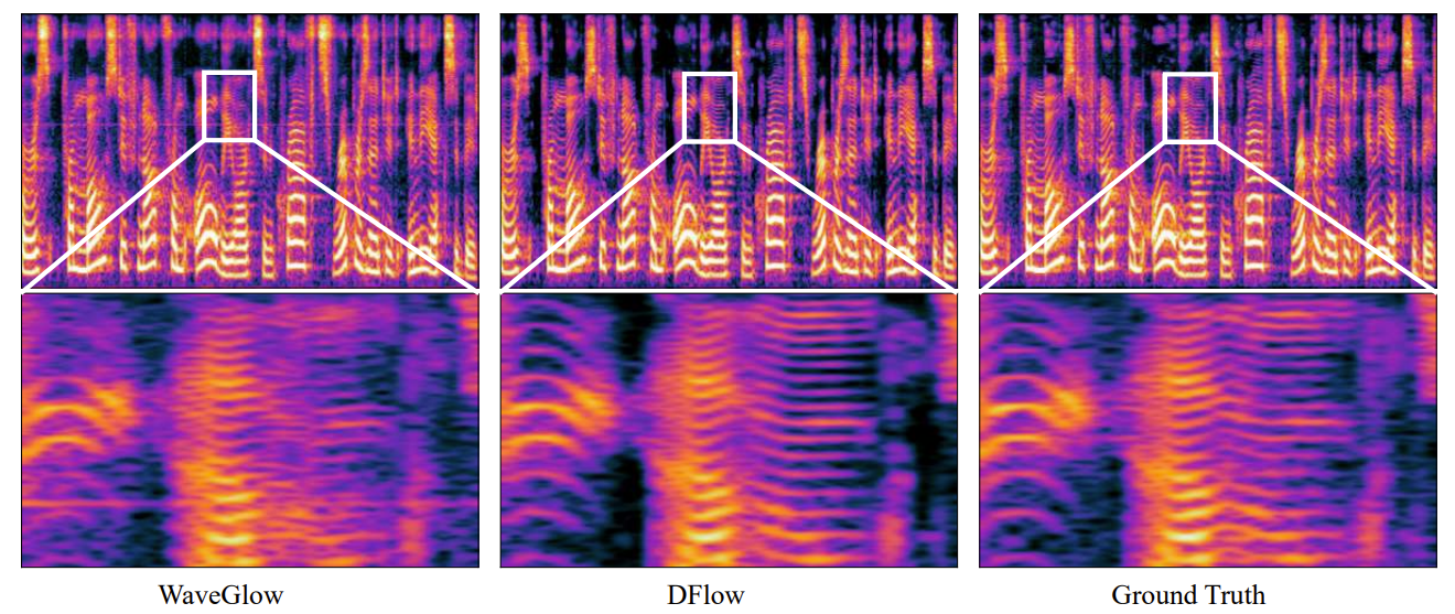
    - 특히 waveform generation에서 time-domain signal의 likelihood는 human perception에 대해 unconsistent한 반면, frequency-domain information은 human perception과 크게 관련되어 있음
  • 이때 time-domain의 minor variation은 frequency-domain에서 perceptible 한 변화를 유발할 수 있음
    1. 실제로 아래 그림과 같이, frequency-domain에서 WaveGlow로 생성된 waveform의 harmonic component는 ground-truth에 비해 blurry 하게 나타남
    2. 따라서 high-fidelity waveform generation을 보장하기 위해서는, NF model이 input data의 small change에 대해서도 충분히 robust 해야 함
  • 추가적으로 NF model은 $p(f_{\theta }(x)),p(z)$ 간의 mismatch로 인한 initial error 문제가 존재함
    - 해당 initial error는 input data의 minor variation에 대한 distinct output을 발생시키는 원인
  • 특히 WaveGlow나 WaveFlow는 Affine Coupling layer에서 Squeeze operation을 채택해 1-dimensional waveform을 multi-dimensional vector로 변환함
    - BUT, 해당 periodic operation은 training 중에 $p(f_{\theta }(x))$에 bias를 추가하므로 sampling 중에 나타나는 initial error로 인해 output waveform에 periodic artifact가 발생할 수 있음

Mel-spectrogram 비교

3. Method

- Overview

• 앞선 standard NF의 한계를 극복하기 위해서는 standard NF의 capacity를 향상하는 refinement module을 train 해야 함
  • 이를 위해 논문은 complex data distribution $p(\mathbf{x})$에 대한 generation을 2단계로 나눔:
    1. Generation step
       - Noisy data distribution $p(\tilde{\mathbf{x}})$를 학습
    2. Refinement step
       - Noisy data distribution $p(\mathbf{x}|\tilde{\mathbf{x}})$에 기반하여 clean data distribution을 학습
  • 이때 noisy data $\tilde{\mathbf{x}}$는 $\tilde{\mathbf{x}}=\mathbf{x}+\beta ϵ$과 같이 각 clean data sample에 small scalar $\beta$를 가지는 random Gaussian noise $ϵ$을 추가하여 얻어짐
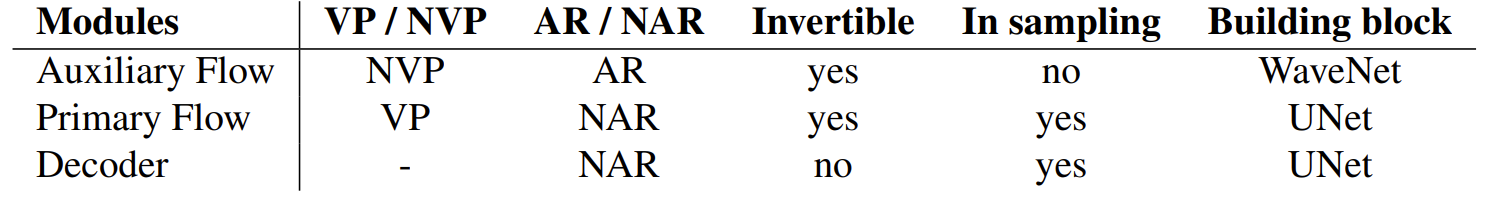
    - $p(\tilde{\mathbf{x}})$의 generation은 NF model로 formulate 되고, refinement step $p(\mathbf{x}|\tilde{\mathbf{x}})$는 DAE로 formulate 됨
  • 구조적으로 DFlow는 Auxiliary Flow network $f$, Primary Flow network $g$, Decoder $m$의 3가지 module로 구성됨
    1. Auxiliary Flow와 Primary Flow는 noisy input $\tilde{\mathbf{x}}$에서 Gaussian prior ${\mathbf{z}}_p$로의 invertible transformation을 수행하는 standard NF를 formulate 함
    2. 이때 Auxiliary Flow는 noisy input $\tilde{\mathbf{x}}$를 latent variable ${\mathbf{z}}_l$로 변환하는 DAE encoder의 역할도 수행함
       
    3. 이로부터 DAE decoder $m$은 clean signal을 reconstruct 하는 방법을 학습함
  • Sampling은 Primary Flow module을 ${\mathbf{z}}_l=g^{-1}({\mathbf{z}}_p)$과 같이 invert 하여 수행되고, 이후 decoder를 통해 output $\hat{\mathbf{x}}=m({\mathbf{z}}_l)$을 생성함
    - 이때 Auxiliary Flow module $f$는 sampling phase에서 제외됨

DFlow Architecture

- Training Objective

• Probabilistic generative modeling은 model parameter $\theta$에 대해 각 training sample $\mathbf{x}\in X$의 marginal log-likelihood를 최대화하는 것을 목표로 함
  • 이를 위해서는 model의 모든 latent variable을 marginalization 해야 함:
    (Eq. 2) $\log p_{\theta }(\mathbf{x})=\log \int p_{\theta }({\mathbf{z}}_l)p_{\theta }(\mathbf{x}|{\mathbf{z}}_l)d{\mathbf{z}}_l$
    - $\theta$ : network $g$와 $m$의 generative parameter
    
  • Auxiliary Flow network $f$는 invertible flow module이므로 (Eq. 2)는 다음과 같이 rewrite 됨:
    (Eq. 3) $\log p_{\theta }(\mathbf{x})=\log \int p_{\theta }({\mathbf{z}}_l)p_{\varphi }(\tilde{\mathbf{x}}|{\mathbf{z}}_l)p_{\varphi }({\mathbf{z}}_l|\tilde{\mathbf{x}})p_{\theta }(\mathbf{x}|{\mathbf{z}}_l)d\tilde{\mathbf{x}}=\log \int p_{\theta ,\varphi }(\tilde{\mathbf{x}})p_{\theta ,\varphi }(\mathbf{x}|\tilde{\mathbf{x}})d\tilde{\mathbf{x}}$
    - $\varphi$ : $f$의 parameter
  • 앞선 integration은 intractble 하므로 variational principle에 따라 marginal likelihood의 lower bound를 최적화함:
    (Eq. 4) $\log p_{\theta }(\mathbf{x})=\log \int p_{\theta ,\varphi }(\tilde{\mathbf{x}})p_{\theta ,\varphi }(\mathbf{x}|\tilde{\mathbf{x}})d\tilde{\mathbf{x}}=\log \int \frac{q_{\beta }(\tilde{\mathbf{x}}|\mathbf{x})}{q_{\beta }(\tilde{\mathbf{x}}|\mathbf{x})}{p}_{\theta ,\varphi }(\tilde{\mathbf{x}})p_{\theta ,\varphi }(\mathbf{x}|\tilde{\mathbf{x}})d\tilde{\mathbf{x}}$
    $\ge {\mathbb{E}}_{q_{\beta }(\tilde{\mathbf{x}}|\mathbf{x})}[\log p_{\theta ,\varphi }(\mathbf{x}|\tilde{\mathbf{x}})+\log p_{\theta ,\varphi }(\tilde{\mathbf{x}})-\log q_{\beta }(\tilde{\mathbf{x}}|\mathbf{x})]$
    - 이를 Evidence Lower BOund (ELBO)라 하고, 첫 번째 term은 DAE의 expected negative reconstruction error에 해당함
    - 마지막 두 term은 $D_{KL}(q_{\beta }(\tilde{\mathbf{x}}|\mathbf{x})||p_{\theta ,\varphi }(\tilde{\mathbf{x}}))$와 같이 근사된 posterior와 prior distribution 간의 KL divergence로 결합될 수 있음
  • 이때 $\beta$는 constant이므로 (Eq. 4)의 마지막 term은 training 중에 최적화할 필요가 없고, 결과적으로 training objective는 NF에 의해 제공된 $\tilde{x}$의 negative log-likelihood와 DAE에 의한 reconstruction error ${\mathcal{L}}_{rec}$를 결합하여 얻어짐:
    (Eq. 5) ${\mathcal{L}}_{all}=-\log p(\tilde{\mathbf{x}})+{\mathcal{L}}_{rec}$
• Negative Log-Likelihood
  • (Eq. 1)을 따라 $\tilde{\mathbf{x}}$의 negative log-likelihood (NLL)은 다음과 같이 계산됨:
    (Eq. 6) $-\log p(\tilde{\mathbf{x}})=-\log (p({\mathbf{z}}_p))-\log (|det(J(f))|)-\log (|det(J(g))|)$
    (Eq. 7) $=-\log (p({\mathbf{z}}_p))-\log (|det(J(f))|)$
    - ${\mathbf{z}}_p\sim \mathcal{N}(0,I)$, $det(J(f)),det(J(g))$ : 각각 $f,g$의 Jacobian determinant
  • 여기서 $g$는 VP flow로 설계되므로, $det(J(g))=1$이고 $\log (|det(J(g))|)=0$ 
• Reconstruction Error
  • DAE의 reconstruction error는 예측된 audio $\hat{\mathbf{x}}$와 clean audio $\mathbf{x}$ 간의 Mean Absolute Error (MAE)로 얻어짐 
  • 이때 MAE에 positive scalar $1/\beta$를 곱하여 사용함:
    (Eq. 8) ${\mathcal{L}}_{rec}=\frac{1}{\beta }||\mathbf{x}-\hat{\mathbf{x}}|{|}_1$

- Noise Injection

• Input $\mathbf{x}$에 noise injection이 없는 경우, network $f,m$은 일반적인 AutoEncoder (AE)를 형성하고 이때 decoder는 encoder의 estimated inverse 역할을 수행함
  • BUT, 해당 방식의 $g+m$ generation process는 $g+f$ NF module을 directly invert 하는 것보다 나쁜 성능을 보임
    - 이는 $m$에 의해 제공되는 estimated inverse가 $f$의 exact inverse 보다 덜 정확하기 때문
  • 따라서 DFlow에서는 decoder $m$이 $f$의 estimated inverse 이상의 capability를 가지는 것을 목표로 DAE를 통해 noise를 inject 함
    • 이를 통해 decoder $m$은 exact input 이상을 학습할 수 있으므로, standard NF model 보다 뛰어난 성능을 달성할 수 있음
    • Noise injection을 활용하면 minor input variation에 대해서도 heightened sensistvity와 robustness를 가지는 expressive latent representation을 얻을 수 있음
      - 결과적으로 high-frequency detail generation에 대한 model capability가 개선됨
    • 추가적으로 decoder는 추론 중에 Primary Flow network의 inverting으로 발생하는 minor error에 대응할 수 있으므로 생성 품질을 더욱 향상할 수 있음

- Auxiliary Flow

• Auxiliary flow $f$는 invertible AR transformation의 stack으로 구성되어 standard NF와 DAE encoder 역할을 수행함
  • 이때 DFlow의 invertible encoder는 Jacobian determinant에 대한 explicit computing을 제공하므로 fixed distribution을 가지는 observed variable인 $\tilde{\mathbf{x}}$에 대해 standard NF를 directly train 할 수 있도록 함 
    1. 예시로 standard NF가 AE의 latent variable에 대해 training 되는 Latent Flow Model (LFM)은 training 이전에 latent space variable을 개별적으로 학습해야 하는 한계가 있음
       
    2. 반면 DFlow는 LFM과 달리 fixed distribution에 대한 log-likelihood를 계산하므로 LFM의 training stability 문제를 극복 가능
       - 특히 DFlow는 $f$가 sampling process에서 완전히 제외되므로 $f$ inverting에 대한 문제를 완전히 무시할 수 있음
  • 결과적으로 DFlow는 다음의 장점을 가지는 autoregressive AR transformation을 사용하여 $f$를 구성함:
    1. Invertible AR transformation은 NAR transformation보다 훨씬 expressive 하고 더 적은 수의 layer를 가짐
    2. AR transformation에는 성능 저하를 일으킬 수 있는 Squeeze operation이 필요하지 않음
    3. Causal convolution을 활용한 AR transformation은 parallel training이 가능함
  • 구조적으로 Auxiliary Flow는 left-to-right block과 right-to-left block으로 구성되어 bidirection으로 inductive bias를 exhibit 할 수 있음 
    1. 이때 각 block에는 다음과 같은 4개의 single-directional AR transformation이 포함됨:
       (Eq. 9) $\log s_i,b_i,{\mathbf{h}}_i^{\prime }=\text{WaveNet}({\mathbf{x}}_{1:i-1},{\mathbf{h}}_{1:i-1})$
       (Eq. 10) ${\mathbf{x}}_i^{\prime }=s_i\cdot {\mathbf{x}}_i+b_i$
       - $\text{WaveNet}(\cdot ,\cdot )$ : standard causal WaveNet block, $\mathbf{h}\in {\mathcal{R}}^{D_h\times T}$ : dimension $D_h$를 가지는 hidden variable
    2. 각 block에 대해 $\mathbf{h}$는 zero-vector로 initialize되고 해당 block 내의 모든 AR transformation을 통해 전달됨
    3. Variable ${\mathbf{h}}_i$는 previous sample ${\mathbf{x}}_{1:i-1}$에서 파생되므로 Jacobian determinant에 영향을 주지 않음
       - 즉, $\frac{\partial {\mathbf{h}}_i}{\partial {\mathbf{x}}_i}=0$
  • 한편으로 논문은 한 transformation에서 다음 transformation으로 extensive information을 전달할 수 있도록 $D_h\gg 1$로 설정함
    - 결과적으로 이를 통해 NF-based model의 bottleneck 문제를 해결 가능

Model Details

- Primary Flow

• Stable training 외에도, final output $\hat{\mathbf{x}}$는 ${\mathbf{z}}_l$에서 파생되므로 expressive 한 latent variable ${\mathbf{z}}_l$을 얻는 것도 중요함 
  • 이를 위해 Primary Flow $g$는 VP flow를 기반으로 설계됨 
    1. 만약 $f,g$가 모두 NVP flow이면 $\hat{\mathbf{x}}$의 NLL은 (Eq. 7)이 아닌 (Eq. 6)이 되고, $f$의 Jacobian determinant를 최대화하는데 대한 constraint는 NLL에 대한 (Eq. 6)의 extra term으로 인해 weakening 됨
    2. 이 경우 $f$는 latent space에 대해 force 되지 않으므로 ${\mathbf{z}}_l$은 small variance를 가지게 되고, 결과적으로 expressiveness가 저하됨
       - Training 역시 ${\mathbf{z}}_l$이 under-constrained 하므로 unstable 하고 reconstruction process에 크게 의존하게 됨
  • 따라서 논문은 $g$를 Volume-Preseving (VP)로 constraining 함으로써, ${\mathbf{z}}_l,{\mathbf{z}}_p$가 동일한 variance를 가지도록 보장해 ${\mathbf{z}}_l$에 대한 regularization constraint를 적용함
    - 추가적으로 volume-preserving constraint는 $f$가 variance가 있는 ${\mathbf{z}}_l$을 생성하도록 유도하여 expressiveness를 크게 향상할 수 있음
  • 구체적으로, DFlow에서는 squeeze layer를 사용하여 1-dimensional latent variable ${\mathbf{z}}_l\in {\mathcal{R}}^{1\times T}$를 4-dimensional vector ${\mathbf{z}}_l^{\prime }\in {\mathcal{R}}^{4\times T/4}$로 rearrange 함 
    1. 이후 squeezed vector ${\mathbf{z}}_l^{\prime }$은 additive coupling layer stack으로 전달되고, channel order는 각 coupling layer 다음의 flip layer를 통해 reverse 됨
    2. 여기서 additive coupling layer의 효율성을 위해, $\text{UNet}(\cdot )$ structure를 통해 additive coupling을 parameterize 함:
       (Eq. 11) ${\mathbf{x}}_1,{\mathbf{x}}_2=\text{Split}(\mathbf{x}),\mathbf{b}=\text{UNet}({\mathbf{x}}_2)$
       (Eq. 12) ${\mathbf{x}}_1^{\prime }={\mathbf{x}}_1+\mathbf{b},{\mathbf{x}}_2^{\prime }={\mathbf{x}}_2,{\mathbf{x}}^{\prime }=\text{Concat}({\mathbf{x}}_1^{\prime },{\mathbf{x}}_2^{\prime })$
  • 구조적으로 $\text{UNet}(\cdot )$ structure는 위 그림과 같이 downsampling stage와 upsampling stage로 구성됨 
    1. 이때 3개의 strided convolution layer와 3개의 transposed convolution layer를 각각 down/upsampling process에 사용하고, 모든 single layer 사이에는 dilated convolution 기반의 residual block을 포함함
    2. Input vector는 $(4,4,4)$ factor로 downsampling 한 다음, 동일한 factor로 upsampling 함
       - 여기서 각 residual block의 channel size는 2배씩 증가/감소함

- Decoder

• Decoder $m$은 U-Net layer series를 기반으로 invertible 되지 않는 feed-forward convolution layer stack으로 구성됨
  • 해당 U-Net layer는 large-scale receptive field를 통해 high-resolution, high-quality waveform generation을 위한 inductive bias를 모델에 제공함
  • 이때 추가적으로 tanh activation을 final output에 적용

DFlow Module 구성

4. Experiments

- Settings

• Dataset : VCTK
• Comparisons : WaveNet, WaveGlow, HiFi-GAN, DiffWave, BigVGAN

- Results

• 전체적인 성능 측면에서 DFlow는 가장 우수한 결과를 보임

모델 성능 비교

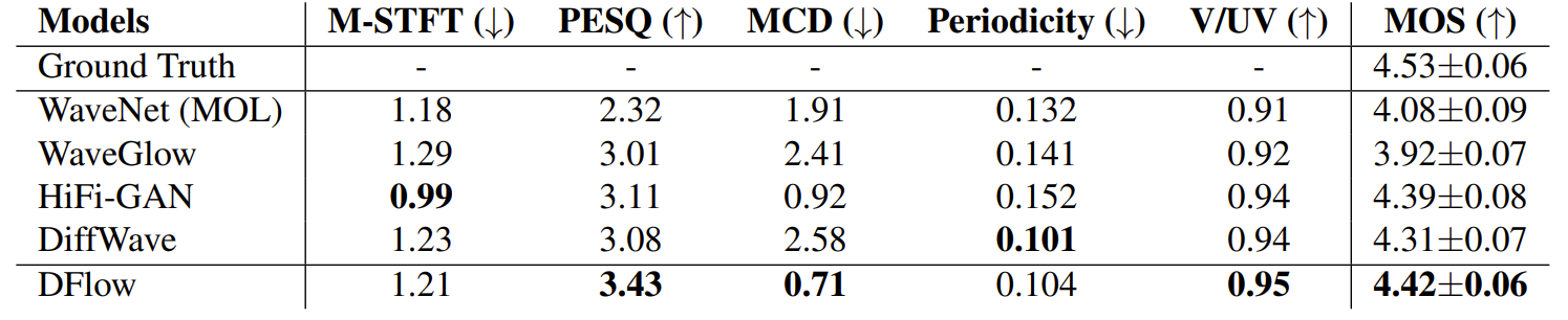
• DFlow는 105.3M의 parameter 수에도 불구하고 HiFi-GAN 수준의 빠른 RTF를 달성함

Efficiency 비교

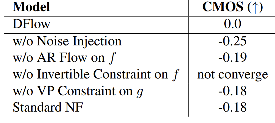
• Ablation Study
  • Ablation study 측면에서 각 component를 제거하는 경우 성능 저하가 발생함
  • 특히 invertible constraint가 사용되지 않으면 모델이 수렴하지 않음

Ablation Study 결과

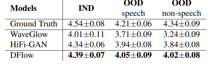
• Generalization on OOD Samples
  • DFlow의 generalization ability를 확인하기 위해 Multilingual TEDx Corpus, MUSDB18-HQ dataset을 사용하여 OOD sample을 구성
  • 결과적으로 DFlow는 OOD test set에서도 가장 우수한 성능을 달성함

OOD Sample에 대한 성능 비교

• DFlow with Large-Scale Training
  • Primary Flow의 invertible layer와 Decoder의 U-Net layer를 조정하여 big model인 DFlow-XL, DFlow-L을 얻음
  • 결과적으로 얻어진 DFlow-XL은 BigVGAN 보다 높은 성능을 보임

Large-Scale Training에 대한 성능 비교