[Paper 리뷰] FreGrad: Lightweight and Fast Frequency-aware Diffusion Vocoder

FreGrad: Lightweight and Fast Frequency-aware Diffusion Vocoder

---

• Lightweight, fast diffusion-based vocoder를 사용하여 사실적인 audio를 합성할 필요가 있음
• FreGrad
  • 복잡한 waveform을 sub-band wavelet으로 decompose 하는 discrete wavelet transform을 적용
  • Frequency awareness를 높이는 frequency-aware dilated convolution을 도입
  • 합성 품질을 향상할 수 있는 추가적인 bag of tricks를 소개
• 논문 (ICASSP 2024) : Paper Link

---

1. Introduction

• Neural vocoder는 mel-spectrogram과 같은 intermediate acoustic feature에서 audible waveform을 합성하는 것을 목표로 함
  • 일반적으로는 autoregressive (AR) architecture를 활용하지만 sequential operation으로 인해 느린 추론 속도를 보임
  • Flow, Generative Adversarial Network 등을 기반으로 하는 non-AR architecture는 이러한 추론 속도 문제를 해결 가능
    - 여러 non-AR 방식 중에서도 특히 diffusion-based vocoder는 우수한 합성 품질을 보이고 있음
    - BUT, diffusion-based vocoder의 높은 계산 비용으로 인한 느린 추론 속도 문제는 여전히 해결되지 못함

-> 그래서 고품질의 음성 합성과 빠른 추론 속도를 달성하는 diffusion-based vocoder인 FreGrad를 제안

 

• FreGrad
  • 복잡한 waveform을 2개의 단순한 frequency sub-band sequence로 decompose 하여 계산 비용을 줄임
    - 이를 위해 waveform을 information loss 없이 frequency-sparse, dimension-reduced feature로 변환하는 Discrete Wavelet Transform (DWT)를 활용
  • Output 품질 향상을 위해, Frequency-aware Dilated Convolution (Freq-DConv)를 도입
    - Dilated convolution에 DWT를 incorporating 함으로써 frequency information의 inductive bias를 제공하여 정확한 spectral 분포를 학습할 수 있도록 함
  • 추가적인 품질 향상을 위해 각 wavelet feature에 대한 prior 분포를 설계하고, sub-optimal noise schedule을 대체하는 noise schedule을 incorporate
    - Frequency-aware feedback을 제공하는 multi-resolution magnitude loss도 추가 적용

< Overall of FreGrad >

• 복잡한 waveform을 sub-band wavelet으로 decompose 하는 DWT를 적용
• Frequency awareness를 높이는 frequency-aware dilated convolution을 도입하고, 합성 품질을 향상할 수 있는 추가적인 bag of tricks를 소개
• 결과적으로 FreGrad는 다른 diffusion-based vocoder 보다 더 우수한 합성 품질과 빠른 추론 속도를 달성

FreGrad의 효율성

2. Backgrounds

• Denoising diffusion probabilistic model은 noisy signal을 denoising 하여 data 분포를 학습하는 latent variable 모델
  • Forward process $q(\cdot)$은 Markov process로 parameterize 된 Gaussian transition을 통해 data sample을 diffuse 함:
    (Eq. 1) $q(x_{t}|x_{t-1})=\mathcal{N}(x_{t};\sqrt{1-\beta_{t}}x_{t-1},\beta_{t}I)$
    - $\beta_{t} \in \{ \beta_{1},...,\beta_{T}\}$ : pre-defined noise schedule
    - $T$ : 총 timestep 수, $x_{0}$ : ground-truth sample
  • 위 function을 통해 $x_{0}$에서 $x_{t}$를 sampling 할 수 있고, 이는 다음과 같이 공식화됨:
    (Eq. 2) $x_{t}=\sqrt{\gamma_{t}}x_{0}+\sqrt{1-\gamma_{t}}\epsilon$
    - $\gamma_{t} =\prod_{i=1}^{t} (1-\beta_{i})$, $\epsilon \sim \mathcal{N}(0,I)$
  • 이때 $T$가 충분히 큰 경우, $x_{T}$의 분포는 isotropic Gaussian 분포에 근사함
    - 결과적으로 initial point $x_{T} \sim \mathcal{N}(0,I)$로부터 exact reverse process $p(x_{t-1}|x_{t})$를 tracing 함으로써 ground-truth 분포의 sample을 얻을 수 있음
    - 여기서 $p(x_{t-1}|x_{t})$는 전체 data 분포에 따라 달라지므로, $\mathcal{N}(x_{t-1};\mu_{\theta}(x_{t},t), \sigma^{2}_{\theta}(x_{t},t))$로 정의되는 neural network $p_{\theta}(x_{t-1}|x_{t})$로 근사
  • 그러면 분산 $\sigma^{2}_{\theta}(\cdot)$는 $\frac{1-\gamma_{t-1}}{1-\gamma_{t}}\beta_{t}$로 표현되고, 평균 $\mu_{\theta}(\cdot)$은:
    (Eq. 3) $\mu_{\theta}(x_{t},t)=\frac{1}{\sqrt{1-\beta_{t}}}\left( x_{t}-\frac{\beta_{t}}{\sqrt{1-\gamma_{t}}}\epsilon_{\theta}(x_{t},t)\right)$
    - $\epsilon(\cdot)$ : noise를 예측하는 neural network
  • $\epsilon_{\theta}(\cdot)$에 대한 training objective는 $\mathbb{E}_{t,x_{t},\epsilon}\left[ || \epsilon-\epsilon_{\theta}(x_{t},t)||_{2}^{2}\right]$를 최소화하도록 simplify 됨
    - 이때 PriorGrad의 경우 prior 분포 $\mathcal{N}(0, \Sigma)$에서 sampling 하는 방식을 도입
    - $\Sigma$는 diagonal matrix $diag\left[(\sigma_{0}^{2},\sigma^{2}_{1},...,\sigma_{N}^{2})\right]$이고, $\sigma^{2}_{i}$는 length $N$을 갖는 mel-spectrogram의 $i$-th normalized frame-level energy
  • 따라서 $\epsilon_{\theta}(\cdot)$에 대한 modified loss function은:
    (Eq. 4) $\mathcal{L}_{diff}=\mathbb{E}_{t,x_{t},\epsilon,c}\left[ || \epsilon-\epsilon_{\theta}(x_{t},t,X)||_{\Sigma^{-1}}^{2} \right]$
    - $||x||_{\Sigma^{-1}}^{2}=x^{T}\Sigma^{-1}x$, $X$ : mel-spectrogram 

3. FreGrad

• FreGrad는 DiffWave를 기반으로 구성됨
  - 대신 concise wavelet feature space에서 동작하고, 기존의 dilated convolution을 Freq-DConv로 대체함

Overall of FreGrad

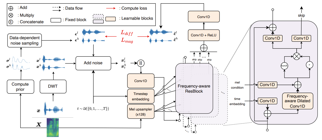
- Wavelet Features Denoising

• Diffusion 모델의 계산량을 줄이기 위해 forward process 이전에 DWT를 적용함
  • DWT는 target dimension audio $x_{0} \in \mathbb{R}^{L}$을 2개의 wavelet feature $\{ x_{0}^{l}, x_{0}^{h} \} \subset \mathbb{R}^{\frac{L}{2}}$로 downsampling 함
    - 각각의 wavelet feature는 low-/high-frequency component를 의미
    - DWT는 biorthogonal property로 인해 information loss 없이 non-stationary signal을 deconstruct 할 수 있음
  • 이를 기반으로 FreGrad는 단순한 wavelet feature로 동작함
    1. 각 training step에서 wavelet feature $x_{0}^{l}, x_{0}^{h}$는 distinct noise $\epsilon^{l}, \epsilon^{h}$를 갖는 timestep $t$에서 noisy feature로 diffuse 되고, 각 noise는 neural network $\epsilon_{\theta}(\cdot)$에 의해 simultaneously approximate 됨
       
    2. Reverse process에서 FreGrad는 denoised wavelet feature $\{ \hat{x}_{0}^{l}, \hat{x}_{0}^{h} \} \subset \mathbb{R}^{\frac{L}{2}}$를 생성하고, inverse DWT (iDWT)에 의해 target waveform $\hat{x}_{0} \in \mathbb{R}^{L}$로 변환됨:
       (Eq. 5) $\hat{x}_{0}=\Phi^{-1}(\hat{x}_{0}^{l}, \hat{x}_{0}^{h})$
       - $\Phi^{-1}(\cdot)$ : iDWT function
  • 결과적으로 FreGrad는 복잡한 waveform에 대한 decomposition을 통해 더 작은 계산량을 가짐
    - iDWT는 wavelet feature로부터 waveform의 lossless reconstruction을 보장하므로 합성 품질을 유지할 수 있음
    - 이를 위해 논문에서는 Haar wavelet을 사용

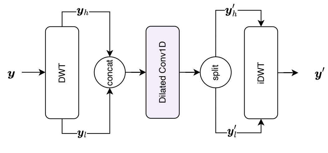
- Frequency-aware Dilated Convolution

• Audio는 다양한 frequency의 mixture이기 때문에, 자연스러운 합성을 위해서는 정확한 frequency 분포를 reconstruct 하는 것이 중요
  • 따라서 FreGrad는 합성 품질 향상을 위해 모델이 frequency information에 집중하도록 deliberately guide 하는 Freq-DConv를 도입
    1. 이를 위해 hidden signal $y\in \mathbb{R}^{\frac{L}{2}\times D}$를 hidden dimension $D$를 갖는 2개의 sub-band $\{ y_{l}, y_{h}\} \subset \mathbb{R}^{\frac{L}{4}\times D}$로 decompose 하는 DWT를 채택
    2. 이후 sub-band는 channel-wise concatenate 되고, dilated convolution $\mathbf{f}(\cdot)$은 frequency-aware feature $y_{hidden} \in \mathbb{R}^{\frac{L}{4} \times 2D}$를 추출:
       (Eq. 6) $y_{hidden}=\mathbf{f}(\textrm{cat}(y_{l},y_{h}))$
       - $\textrm{cat}$ : concatenation operation
    3. 추출된 feature $y_{hidden}$은 channel dimension을 따라 $\{ y'_{l}, y'_{h} \} \subset \mathbb{R}^{\frac{L}{4} \times D}$로 bisect 되고, iDWT는 input feature $y$와 length를 match 하기 위해 abstract feature를 single hidden representation으로 변환:
       (Eq. 7) $y' = \Phi^{-1}(y'_{l},y'_{h})$
       - $y' \in \mathbb{R}^{\frac{L}{2}\times D}$ : Freq-DConv의 output
       - Freq-DConv는 모든 ResBlock에 embed 됨
  • Dilated convolution 이전에 hidden signal을 decompose 하는 것은 kernel size를 변경하지 않고 time axis를 따라 receptive field를 늘릴 수 있기 때문
    - DWT로 인해 각 wavelet feature는 모든 temporal correlation을 유지하면서 reduced temporal dimension을 가짐
    - 각 convolution layer가 동일한 kernel size에서도 time dimension을 따라 더 큰 receptive field를 posses 하도록 함
  • 추가적으로 Freq-DConv를 통해 각 hidden feature의 low-/high-frequency sub-band를 개별적으로 explore 할 수 있음
    - 결과적으로 모델에 frequency information의 inductive bias를 제공함으로써 frequency-consistent waveform을 생성

Frequency-aware Dilated Convolution

- Bag of Tricks for Quality

• Prior Distribution
  • Spectrogram-based prior 분포는 더 적은 sampling step으로도 waveform denoising 성능을 크게 개선 가능
  • 따라서 FreGrad는 mel-spectrogram을 기반으로 각 wavelet sequence에 대한 prior 분포를 설계
    - 각 sub-band sequence에는 specific low-/high-frequency information이 포함되어 있으므로, 각 wavelet feature에 대해 개별적인 prior 분포를 사용
    
  • 이를 위해, mel-spectrogram을 frequency dimension을 따라 2개의 segment로 나누고, 각 segment에서 개별적인 prior 분포 $\{\sigma^{l}, \sigma^{h}\}$를 얻음
• Noise Schedule Transformation
  • Signal-to-Noise Ratio (SNR)은 forward process의 final timestep $T$에서 이상적으로 $0$이어야 함
    - BUT, 기존의 noise schedule은 final timestep에서 SNR이 $0$에 도달하지 못함
  • 따라서 $0$ SNR을 달성하기 위해, 다음의 공식화를 활용:
    (Eq. 8) $\sqrt{\gamma}_{new}=\frac{\sqrt{\gamma}_{0}}{\sqrt{\gamma}_{0}-\sqrt{\gamma}_{T}+\tau}(\sqrt{\gamma}-\sqrt{\gamma}_{T}+\tau)$
    - $\tau$ : sampling process에서 $0$으로 나누어지는 것을 방지하는 역할
• Loss Function
  • Diffusion vocoder의 일반적인 training objective는 frequency 측면에서 explicit feedback이 부족한 예측/ground-truth noise 사이의 $L2$ norm을 최소화하는 것
  • 모델에 frequency-aware feedback을 제공하기 위해, FreGrad는 multi-resolution STFT magnitude loss $\mathcal{L}_{mag}$를 추가
    - 이때 spectral convergence loss를 추가하면 경험적으로 output 품질이 저하되기 때문에 magnitude loss만 활용함
  • 여기서 $M$을 STFT loss의 수라고 했을 때, $\mathcal{L}_{mag}$는:
    (Eq. 9) $\mathcal{L}_{mag}=\frac{1}{M}\sum_{i=1}^{M}\mathcal{L}^{(i)}_{mag}$
    - $\mathcal{L}^{(i)}_{mag}$ : $i$-th analysis setting에서 STFT magnitude loss
    
  • 따라서 diffusion loss를 low-/high-frequency sub-band에 개별적으로 적용한 final training objective는:
    (Eq. 10) $\mathcal{L}_{final}=\sum_{i\in\{l,h\}}\left[\mathcal{L}_{diff}(\epsilon^{l},\hat{\epsilon}^{i})+\lambda \mathcal{L}_{mag}(\epsilon^{i},\hat{\epsilon}^{i})\right]$
    - $\hat{\epsilon}$ : estimated noise

Timestep에 따른 Noise Level과 log SNR

4. Experiments

- Settings

• Dataset : LJSpeech
• Comparisons : WaveGrad, DiffWave, PriorGrad

- Results

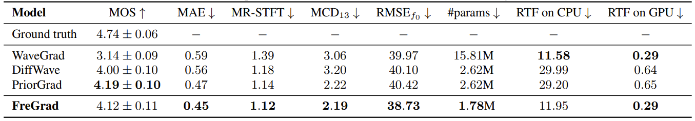
• Audio Quality and Sampling Speed
  • FreGrad는 parameter 수 뿐만 아니라 CPU, GPU 모두에서 추론 속도를 크게 개선함
  • 합성 품질 측면에서도 FreGrad는 가장 우수한 성능을 보임
    - MOS 측면에서는 다소 낮은 성능을 보이는데 이는 low-frequency 분포에 대한 sensitivity 때문

모델 성능 비교

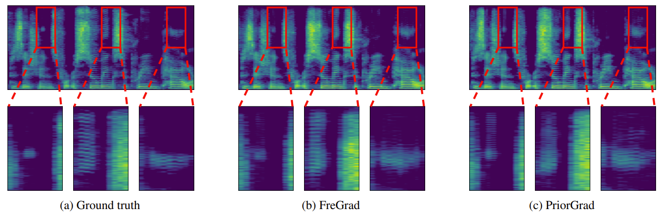
• Mel-spectrogram을 비교해 보면, FreGrad는 정확한 frequency 분포를 reconstruction 할 수 있음

Mel-spectrogram 비교

• Ablation Study
  • 논문에서 제안된 각 component는 FreGrad의 합성 품질을 향상하는데 큰 기여를 함
  • 특히 Freq-DConv는 품질을 크게 향상할 수 있고, $\mathcal {L}_{mag}$의 경우 frequency-aware feedback에 중요한 역할을 함

Ablation Study 결과