[Paper 리뷰] SiD-WaveFlow: A Low-Resource Vocoder Independent of Prior Knowledge

SiD-WaveFlow: A Low-Resource Vocoder Independent of Prior Knowledge

---

• Flow-based nerual vocoder는 high-fidelity의 음성을 합성할 수 있지만, training에 많은 speech data가 필요하고 computationally heavy 함
• SiD-WaveFlow
  • Low-resource 합성을 위한 flow-based neural vocoder
  • WaveGlow의 Affine Coupling Layer의 계산 효율성을 개선하기 위해 Semi-inverse Dynamic Transformation module을 도입
• 논문 (INTERSPEECH 2022) : Paper Link

---

1. Introduction

• Vocoder는 mel-spectrogram과 같은 acoustic feature로부터 waveform을 합성하는 것을 목표로 함
  • 최근에는 generative network를 활용하는 neural vocoder가 뛰어난 합성 성능을 보이고 있고, 크게 autoregressive, non-autoregressive 방식으로 나누어짐
  • 특히 non-autoregressive 방식은 autoregressive 모델보다 빠른 추론 속도를 달성할 수 있다는 장점이 있음
    - BUT, 여전히 structural complexity로 인해 training을 위한 많은 data와 computation resource가 요구됨
  • WaveGlow, WaveFlow와 같은 flow-based vocoder는 대표적인 non-autoregressive 방식으로 probability density를 invertible mapping의 sequence로 변환함
    1. 여기서 flow-based vocoder는 크게 autoregressive flow 또는 bipartite transform을 주로 활용함 
    2. Bipartite transform은 autoregressive flow 보다 간단한 training pipeline을 가짐
       - BUT, structural complexity로 인해 학습에 여전히 많은 data가 필요하고, 본질적으로 computationally-intensive 하기 때문에 resource-limited 환경에서 사용하기 어려움

-> 그래서 low-resource 환경에서 동작 가능한 효율적인 flow-based vocoder인 SiD-WaveFlow를 제안

 

• SiD-WaveFlow
  • Low-resource condition에서 합성을 수행하기 위해, external knowledge 없이 5분 분량의 speech 만을 사용하여 training 되는 flow-based vocoder
  • Bipartite transform에서 사용되는 Affine Coupling Layer (ACL)을 대체하는 Semi-inverse Dynamic Transform (SiDT) layer를 도입
    - 기존 ACL과 비교하여 SiDT는 더 computationally efficient 하고 빠른 수렴을 지원함
  • Pre-emphasis와 squeeze operation을 포함하는 Prenet module을 추가하여 합성 품질을 추가적으로 개선

< Overall of SiD-WaveFlow >

• Additional information 없이 5분 분량의 speech 만으로 training이 가능하고, 기존 flow-based vocoder에 비해 더 적은 parameter와 computational cost를 가짐
• 결과적으로 빠른 수렴/추론 속도를 달성하면서 Raspberry Pi와 같은 edge-device에서 효과적으로 동작 가능

2. Method

- Preliminaries

• Normalizing flow는 invertible bijective transformation function의 sequence를 통해 normalized density distribution을 target density distribution으로 변환함
  • 즉, flow-based vocoder는 transformation $\mathbf{y}=\mathbf{g}_{1}\circ \mathbf{g}_{2}\circ ... \mathbf{g}_{k}(x)$에 기반해 input mel-spectroram $\mathbf{x}$에 invertible deep neural network $\mathbf{g}_{i}$의 series를 적용하는 방식으로 speech $\mathbf{y}$를 생성함 
  • 여기서 $\mathbf{g}_{i}$는 variable rule에 따라 invertible 하므로, 다음의 negative log-likelihood를 최소화하여 모델을 training 함:
    (Eq. 1) $\log p(\mathbf{y})=\log p(\mathbf{x})+\sum_{i=1}^{K}\log \left| \det \frac{d\mathbf{g}_{i}^{-1}}{d\mathbf{g}_{i-1}^{-1}}\right|$
    - $K$ : invertible mapping 수, $\det \frac{d\mathbf{g}_{i}^{-1}}{d\mathbf{g}_{i-1}^{-1}}$ : $\mathbf{g}^{-1}_{i}$의 Jacobian determinant
  • 여기서 $\mathbf{g}_{i}$가 invertible 하면 $\mathbf{x}$는 $\mathbf{x}=\mathbf{g}_{K}^{-1}\circ \mathbf{g}_{K-1}^{-1}\circ ... \circ \mathbf{g}_{1}^{-1}(\mathbf{y})$와 같이 추론되므로, $\mathbf{g}_{0}^{-1}(\mathbf{y})$는 $\mathbf{y}$와 동일함 
  • 대표적으로 WaveGlow는 위의 invertible transform을 구현하기 위해, squeeze operation, invertible $1\times 1$ convolution module, ACL module로 구성된 structure를 채택함
    1. Invertible $1\times 1$ convolution module과 ACL module은 모델 training과 speech generation 중에 repeat 되어 flow step을 형성
    2. 결과적으로 해당 module을 통해 순차적으로 mel-spectrogram을 speech waveform으로 변환

- Overview of SiD-WaveFlow

• SiD-WaveFlow는 아래 그림과 같이 Prenet module, $K$번 repeat 되는 flow step, split operation으로 구성됨
  • 특히 $K$ step의 flow와 split operation은 training 속도를 가속하기 위해, $T$-scale architecture를 활용
  • Training stage에서
    1. 먼저 speech sample은 Prenet module에 input 됨
    2. 이후 preprocessed speech sample은 $K$번 repeat 되는 flow step으로 전달됨
       - 해당 flow step은 invertible $1\times 1$ convolution layer, SiDT layer의 두 invertible transformation으로 구성됨
       
    3. 최종적으로 $K$ step의 flow를 split 하여 loss를 계산함

Overall of SiD-WaveFlow

- Prenet

• Prenet module에서는 input speech에 대해 pre-emphasis와 squeeze operation을 적용함
  • 먼저, original speech는 high-frequency resolution을 강조하기 위해 pre-emphasis 됨:
    (Eq. 2) $x'(n)=x(n)-ax(n-1)$
    - $x(n), x'(n)$ : 각각 pre-emphasis 전후의 $n$-th sampling point, $a$ : coefficient value (0.9~1)
  • 다음으로 WaveGlow의 squeeze operation을 적용하여 parallel computing을 위한 channel 수를 늘림
    - 즉, pre-emphasized speech sampling vector는 $N\times 1$에서 $\frac{N}{8}\times 8$로 reshape 됨
    - $N$ : sampling point 수

- Semi-inverse Dynamic Transformation

• Affine Coupling Layer (ACL)은 invertible neural network의 series로 normalizing flow를 구현하기 위해 채택되었지만, computational complexity의 한계가 있음
  • 따라서 SiD-WaveFlow는 inverse Dynamic Linear Transformation (iDLT)에 기반한 Semi-inverse Dynamic Transformation (SiDT)로 ACL을 대체함
  • 해당 SiDT는 아래와 같이 정의되어 flow step을 구현하고, 보다 효율적으로 동작 가능함:
    (Eq. 3) $(\mathbf{u}_{1},\mathbf{u}_{2})=\mathrm{split}(\mathbf{u}),\,\, \mathbf{v}_{0}=0$
    (Eq. 4) $(\mathbf{s}_{1},\mathbf{t}_{1})=\mathrm{NN}(\mathbf{m}(\mathbf{v}_{0}),\mathbf{h})$
    (Eq. 5) $\mathbf{v}_{1}=\mathbf{s}_{1}\odot \mathbf{u}_{1}+\mathbf{t}_{1}$
    (Eq. 6) $(\mathbf{s}_{2},\mathbf{t}_{2})=\mathrm{NN}(\mathbf{m}(\mathbf{v}_{1},\mathbf{u}_{1}),\mathbf{h})$
    (Eq. 7) $\mathbf{v}_{2}=\mathbf{s}_{2}\odot \mathbf{u}_{2}+\mathbf{t}_{2}$
    (Eq. 8) $\mathbf{v}=\mathrm{concat}(\mathbf{v}_{1},\mathbf{v}_{2})$
    - $\mathbf{u}$ : input vector, $\mathbf{u}_{1}, \mathbf{u}_{2}$ : vector $\mathbf{u}$를 equally dividing 하여 얻은 vector
    - $\mathbf{v}_{0}$ : zero-vector, $\mathbf{h}$ : SiDT의 ouptut을 adjust 하는 데 사용되는 input speech의 upsampled mel-spectrogram
    - $\mathbf{m}$ : addition/multiplication과 같은 transformation, $\mathrm{NN}(\cdot)$ : modified gated convolution layer
    - $\mathbf{s}_{1}, \mathbf{s}_{2}, \mathbf{t}_{1}, \mathbf{t}_{2}$ : $\mathrm{NN}(\cdot)$에 의해 계산된 affine factor vector
  • 여기서 vector $\mathbf{v}_{1}, \mathbf{v}_{2}$는 (Eq. 5), (Eq. 7)을 사용하여 $\mathbf{s}_{1},\mathbf{s}_{2}, \mathbf{t}_{1},\mathbf{t}_{2}$로부터 계산되고, 최종적으로 output vector $\mathbf{v}$는 $\mathbf{v}_{1}, \mathbf{v}_{2}$를 horizontally concatenate 하여 얻어짐
  • $\mathbf{v}_{0}$는 iDLT와 달리 의도적으로 extra input으로 추가되므로 possible noise interference를 회피하기 위해 zero-vector로 initialize 됨
    1. 특히 $\mathrm{NN}(\cdot)$의 intermediate channel 수가 줄어드므로 information bottleneck의 영향을 완화할 수 있음
    2. 이때 $\mathbf{m}(x,y)$는 parameter 수를 줄이고 계산을 가속화하기 위해, $\mathbf{m}(x,y)=x+y$와 같이 정의됨
    3. 결과적으로 SiDT의 training loss는:
       (Eq. 9) $\log \left| \det \frac{d\mathbf{g}_{SiDT}^{-1}(\mathbf{u})}{d\mathbf{u}}\right|=\log |\mathbf{s}_{1}|+\log |\mathbf{s}_{2}|$
       

- Invertible $1\times 1$ Convolution Layer

• Flow-based generative network는 invertible $1\times 1$ convolutio을 통해 channel order를 reorganize 함
  • 따라서 논문은 $1\times 1$ convolution layer를 SiDT layer 앞에 추가하여 SiD-WaveFlow의 intermediate variable의 order를 reorganize 함
    - 여기서 network의 invertibility를 보장하기 위해 convolution weight $W$는 random orthogonal matrix로 initialize 됨
  • Training 시에 invertible $1\times 1$ convolution layer의 data transformation은 $\mathbf{g}_{1\times 1 \, conv}^{-1}=W\mathbf{z}$로 정의할 수 있음
    - $\mathbf{z}$ : Prenet module의 output / 이전 flow step의 SiDT output vector
  • 결과적으로 invertible $1\times 1$ convolution의 training loss는:
    (Eq. 10) $\log \left| \det \frac{d\mathbf{g}^{-1}_{1\times 1\, conv}(\mathbf{z})}{d\mathbf{z}}\right|=\log |\det W|$
    - $\det \frac{d\mathbf{g}^{-1}_{1\times 1\, conv}(\mathbf{z})}{d\mathbf{z}}$ : invertible $1\times 1$ convolution의 Jacobina determinant

- Multi-Scale Architecture

• Multi-scale architecture는 다양한 time scale에서 information을 추출하고, flow-based model의 학습 속도를 가속할 수 있음
  • 특히 SiD-WaveFlow architecture에는 $T$-scale이 포함되어 있고, 각 scale에는 $K$ step flow가 포함되어 있음
  • Training stage에서 vector의 처음 두 dimension은 split 되어 각 scale의 마지막에서 loss를 계산하고, 나머지 dimension은 다음 scale에 input 됨
    - 최종적으로 $T$-scale 이후, 모든 dimension이 concatenate 되어 SiD-WaveFlow의 output을 생성함
  • 이때 multi-scale structure의 operation은 다음과 같이 정의됨:
    (Eq. 11) $\mathbf{h}_{0}=\mathbf{r}$
    (Eq. 12) $(\mathbf{x}_{i},\mathbf{h}_{i})=\mathrm{split}(\mathrm{Flow}(\mathbf{h}_{i-1}))$
    (Eq. 13) $\mathbf{x}=\mathrm{concat}(\mathbf{x}_{1},\mathbf{x}_{2},...,\mathbf{x}_{T})$
    - $\mathbf{r}$ : Prenet module의 output vector, $\mathrm{Flow}()$ : $K$ step의 flow transformation
    - $\mathrm{split}()$ : $K$ step의 flow에서 $\mathbf{x}_{i}$를 추출하는 split operation 
    - $\mathbf{h}_{i}$ : SiD-WaveFlow의 intermediate vector, $\mathbf{x}$ : training 이후의 output mel-spectrogram
    - 추가적으로 $\mathbf{h}_{0}$는 $\mathbf{r}$로 initialize 됨

3. Experiments

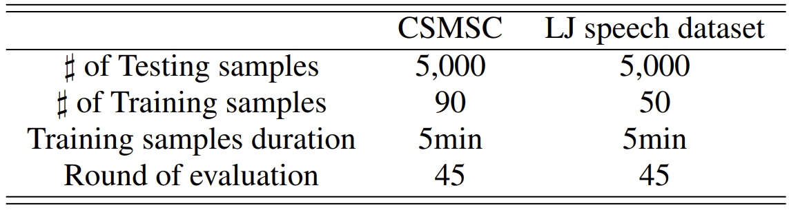
- Settings

• Dataset : CSMSC, LJSpeech
• Comparisons : WaveGlow, Wave-IDLT

Dataset 요약

- Results

• 먼저 MOS 측면에서 SiD-WaveFlow는 가장 뛰어난 성능을 보임

모델 성능 비교

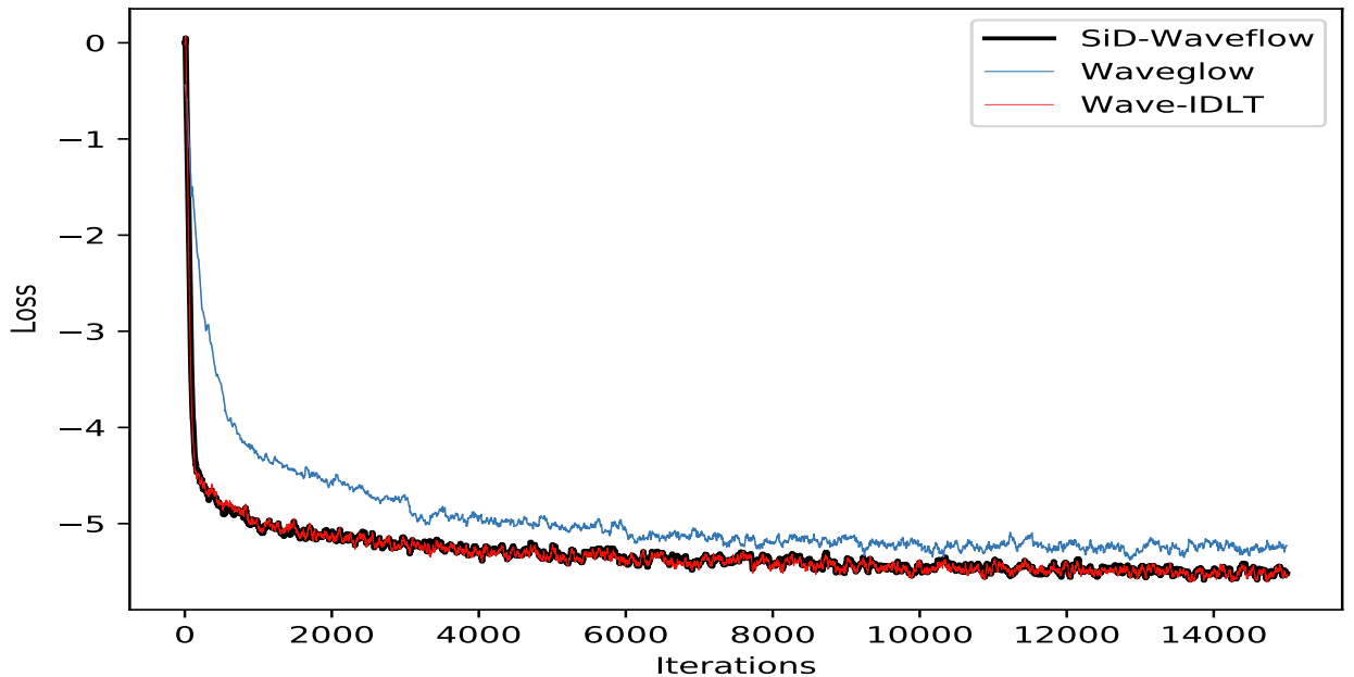
• SiD-WaveFlow는 기존 방식보다 더 빠르게 수렴함

수렴에 필요한 Step 수 비교

Training loss 비교

• 추론 측면에서도, SiD-WaveFlow는 workstation, Raspberry Pi 모두에서 적은 parameter로 동작 가능하면서 가장 빠른 속도를 달성함

추론 속도와 Parameter 수 비교

• Ablation study 측면에서, pre-emphasis를 사용하는 것이 MOS를 더 향상할 수 있는 것으로 나타남

Ablation Study 결과