[Paper 리뷰] EDM2: Analyzing and Improving the Training Dynamics of Diffusion Models

EDM2: Analyzing and Improving the Training Dynamics of Diffusion Models

---

• Diffusion model은 data-driven image synthesis에서 우수한 성능을 보임
• EDM2
  • Diffusion model architecture에 대한 uneven, inefficient training의 원인을 파악
  • Activation, weight, update magnitude를 expectation에 대해 preserve 하도록 network layer를 redesign
  • 추가적으로 training 이후 Exponential Moving Average parameter를 post-hoc setting
• 논문 (CVPR 2024) : Paper Link

---

1. Introduction

• Denoise Diffusion Model은 high-quality image synthesis를 지원함
  • 이때 diffusion model은 pure noise를 iterative image denoising을 통해 새로운 image로 변환함
    - 각 denoising step은 self-attention layer를 가지는 U-Net architecture를 통해 수행됨
  • BUT, diffusion model training은 stochastic loss function으로 인한 어려움이 있음
    
    1. Final image quality는 sampling chain을 통해 predict 되는 faint image detail을 통해 결정되기 때문
    2. Network는 다양한 noise level, Gaussian noise realization, conditioning input 등을 고려해야 하기 때문
       

Complexity 비교

-> 그래서 diffusion model의 predictable, even parameter update를 위한 training dynamics를 조사

 

• EDM2
  • Weight, activation, gradient, weight update에 대한 expected magnitude를 활용
  • 추가적으로 training 이후 Exponential Moving Average (EMA) paramter를 post-hoc setting

< Overall of EDM2 >

• 효과적인 diffusion model training을 위한 training dynamics 분석
• 결과적으로 기존보다 우수한 성능을 달성

2. Improving the Training Dynamics

• 논문은 score network의 training dynamics에서 발생하는 imbalance의 영향을 분석하고 완화하는 것을 목표로 함
  • 먼저 논문은 EDM을 따라 U-Net, self-attention layer로 구성된 ADM network를 채택하고 constant learning rate과 32 deterministic 2nd order sampling step을 사용함
  • Evaluation은 ImageNet $512\times 512$ dataset을 사용함

Changes

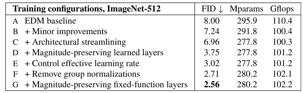
- Preliminary Changes

• Baseline ($\texttt{Config A}$)
  • Original EDM configuration과 달리 output channel을 $4$로 늘림
  • 추가적으로 training dataset을 ImageNet-512의 $64\times 64\times 4$ latent representation으로 replace 하고 zero mean, standard deviation $\sigma_{data}=0.5$로 globally standardize 함
    - 이때 baseline의 FID는 $8.00$으로 얻어짐
• Improved Baseline ($\texttt{Config B}$)
  • Baseline의 성능을 최적화하기 위해 hyperparameter (learning rate, EMA length, training noise level distribution 등)을 tuning 함
    - $32\times 32$ resolution에서는 self-attention을 disable 함
  • 한편 EDM에서는 initialization 시 loss magnitude를 모든 noise level에서 $1.0$으로 standardize 하지만, training progress에서는 hold 되지 않음
    1. 이로 인해 gradient feedback의 magnitude가 noise level에 따라 달라짐
    2. 따라서 논문은 multi-task loss의 continuous generalization을 채택하여 noise level function으로 raw loss value를 track 하고, training loss를 해당 reciprocal로 scalining 함 
  • 결과적으로 $\texttt{Config B}$를 통해 FID는 $8.00$에서 $7.24$로 개선됨 
• Architectural Streamlining ($\texttt{Config C}$)
  • 모든 convolutional, linear layer에서 additive bias를 remove 하고 network의 data offset capability를 보장하기 위해 additional constant $1$ channel을 network input에 concatentate 함 
    1. 추가적으로 He uniform을 통해 weight를 initialize 하고 positional encoding scheme을 standard Fourier feature로 replace 하고, group normalization layer에서 mean subtraction과 learned scaling을 제거하여 simplify 함 
    2. 한편 training 과정에서 key/query vector의 magnitude growth로 인해 attention map에서 brittle, spiky configuration이 나타날 수 있음
       - 이를 해결하기 위해 vector를 normalize 한 다음 dot product 하는 Cosine Attention을 도입함
  • 결과적으로 $\texttt{Config C}$를 통해 FID는 $7.24$에서 $6.96$으로 개선됨 

Overview

- Standardizing Activation Magnitudes

• $\texttt{Config C}$의 simplified architecture를 기반으로 activation magnitude 문제를 분석해 보면
  • 아래 그림과 같이 $\texttt{Config C}$의 training에서 각 block 내의 activation magnitude는 uncontrollably grow 함
    1. 특히 training 마지막에서도 growth는 tapering off 되거나 stabilize 되지 않음
    2. 이는 ADM network가 구조적으로 encoder/decoder/self-attention block의 residual structure로 인해 normalization이 없는 long signal path를 포함하고 있기 때문
       - 해당 path는 residual branch를 통해 contribution을 accumulate 하고 repeated convolution을 통해 activation을 amplify 하여, network을 unoptimal state에 keeping 함
  • 단순하게 해당 path에 group normalization을 적용하는 것을 고려할 수 있지만, StyleGAN과 같이 excessive normalization은 network의 성능을 저하시키고, 각 layer가 학습을 bypass 하도록 유도할 수 있음
  • 따라서 논문은 data-dependent normalization의 영향력을 줄이기 위해, individual layer와 pathway가 expectation을 기반으로 activation magnitude를 preserve 하도록 함
• Magnitude-Preserving Learned Layers ($\texttt{Config D}$)
  • Expected activation mangitude를 preserve 하기 위해 논문은 각 layer output을 activation magnitude의 expected scaling으로 divide 함
  • 여기서 incoming activation에 agnostic 한 scheme을 찾기 위해 다음의 statistical assumption을 고려함:
    1. 먼저 pixel과 feature map이 mutually uncorrelate 되어 있고 equal standard deviation $\sigma_{act}$를 가진다고 가정하자
       - 여기서 fully-connected, convolutional layer는 하나의 output channel 마다 stacked unit으로 구성된다고 볼 수 있음
    2. 각 unit은 output element를 생성하기 위해 input activation의 일부 subset에 weight vector $\mathbf{w}_{i}\in\mathbb{R}^{n}$의 dot product를 apply 할 수 있음
    3. 그러면 해당 가정 하에서 $i$-th channel의 output feature standard deviation은 $||\mathbf{w}_{i}||_{2}\sigma_{act}$가 되고, 논문은 input activation magnitude를 restore 하기 위해 $||\mathbf{w}_{i}||_{2}$를 channel-wise로 divide 함
       
  • $\texttt{Config D}$의 해당 modification을 통해 아래 그림의 3행과 같이 magnitude drift를 eliminate 할 수 있고, FID를 $6.96$에서 $3.75$로 향상할 수 있음

Training Time Evolution (Activation, Weight Magnitude)

- Standardizing Weights and Updates

• 위 그림에서 $\texttt{Config D}$는 network weight가 grow 하는 경향이 있음
  • Weight를 normalize 하는 경우, loss gradient가 weight vector에 perpendicular 하도록 강제되기 때문
    
  • 따라서 논문은 해당 learning rate를 explicit control 할 수 있는 방법을 고려함
• Controlling Effective Learning Rate ($\texttt{Config E}$)
  • 논문은 forced weight normalization을 통해 weight growth 문제를 해결함
    - 여기서 각 training step 이전에 모든 weight vector $\mathbf{w}_{i}$를 unit variance로 explicitly normalize 함
  • 특히 training 시에는 standard weight normalization을 사용하여 training gradient를 $\mathbf{w}_{i}$가 있는 unit-magnitude hypersphere의 tangent plane으로 project 함
    1. 이를 통해 Adam의 variance estimate는 실제 tangent plane step을 통해 compute 될 수 있고, gradient vector의 to-be erased normal component에 corrput 되지 않을 수 있음
    2. 특히 weight, gradient 간의 correlation이 없다고 하면 각 Adam step은 fixed proportion으로 gradient를 approximately replace 할 수 있음
  • Learning rate를 control 할 때 constant learning rate는 convergence를 induce 하지 않으므로, 논문은 Inverse Square Root learning rate decay schedule $\alpha(t)=\alpha_{ref}/\sqrt{\max(t/t_{ref},1)}$을 채택함
    - $t$ : current training iteration, $\alpha_{ref}, t_{ref}$ : hyperparameter
  • 결과적으로 $\texttt{Config E}$는 training 시 weight, activation magnitude를 successfully preserve 하여 FID를 $3.75$에서 $3.02$로 개선함 

- Removing Group Normalizations ($\texttt{Config F}$)

• Data-dependent group normalization layer를 remove 할 수 있음
  • 이때 network는 어떤 normalization layer 없이도 sucessfully training 될 수 있지만, encoder main path에 weaker pixel normalization layer를 도입하면 더 나은 성능을 얻을 수 있음
  • 특히 $\texttt{Config F}$는 $\texttt{Config D}$의 standardization에 대한 statistical assumption을 violate 하는 corrleation을 counteracte 해야 함
    1. 따라서 논문은 모든 group normalization을 remove 하고 $1/4$를 pixel normalization으로 replace 함
    2. 추가적으로 embedding network의 두 번째 linear layer와 network output의 non-linearity를 remove 하고 residual block의 resampling operation을 combine 함
  • 결과적으로 FID는 $3.02$에서 $2.71$로 개선됨 

- Magnitude-Preserving Fixed-Function Layers ($\texttt{Config G}$)

• Network에는 activation magnitude를 preserve 하지 않는 layer가 여전히 존재함
  • 먼저 Fourier feature의 $\sin, \cos$ function은 unit variance를 가지지 않으므로 $\sqrt{2}$로 scaling 해야 함
    1. SiLU non-linearity는 compensate 되지 않으면 expected unit-variance distribution을 attenuate 함
       - 따라서 논문은 output을 $\mathbb{E}_{x\sim \mathcal{N}(0,1)}[\text{silu}(x)^{2}]^{1/2}\approx 0.596$으로 divide 함
    2. Addition이나 concatenation을 통해 2개의 network branch가 join 되는 경우, 각 branch의 contribution에 따라 magnitude가 영향을 받을 수 있음
       - 이를 위해 addition operation을 weighted sum으로 switch 하여 fixed residual path에는 $30\%$ weight, embedding에는 $50\%$ weight를 주고, 해당 weighted sum의 expected standard deviation을 활용함
  • Standardization 이후에는 activation을 learned amount로 scale 하는 specific place를 identify 해야 함:
    1. 먼저 desired output이 항상 unit-vairance를 가지는 것을 expect 할 수 없으므로 network의 가장 끝에 learned zero-initialized scalar gain을 추가함
    2. 각 residual block 내의 conditioning signal에도 유사한 learned gain을 적용함
  • 해당 final configuration을 통해 FID는 $2.56$으로 향상될 수 있음

3. Post-hoc EMA

• Image synthesis에서 model weight에 대한 Exponential Moving Average (EMA)는 큰 영향을 미침
  - 따라서 논문은 EMA profile을 training 이전에 specify 하지 않고 post-hoc으로 choice 하는 방법을 고려함

- Power Function EMA Profile

• 기존의 EMA는 training parameter $\theta$와 network parameter의 running weighted average $\hat{\theta}_{\beta}$를 maintain 함
  • 각 training step에서 average는 $ \hat{\theta}_{\beta}(t)=\beta\hat{\theta}_{\beta}(t-1)+(1-\beta)\theta(t)$로 update 됨
    - $t$ : current training step, Decay rate는 $\beta$에 의해 결정됨
  • 한편 논문은 exponential decay 대신 power function에 기반한 averaging profile을 사용함
    1. Long exponential EMA는 network parameter가 mostly random인 initial training stage에 non-negligible weight를 주는 경향이 있기 때문
    2. Average profile은 training time에 따라 automatically scale 될 수 있기 때문
  • Power function을 사용하면 앞선 요구사항을 반영할 수 있고, 이때 time $t$에서의 averaged parameter를 다음과 같이 정의할 수 있음:
    (Eq. 1) $\hat{\theta}_{\gamma}(t)=\frac{\int_{0}^{t}\tau^{\gamma}\theta(\tau)d\tau}{\int_{0}^{t}\tau^{\gamma}d\tau}=\frac{\gamma+1}{t^{\gamma+1}}\int_{0}^{t}\tau^{\gamma}\theta(\tau)d\tau$
    - $\gamma$ : profile의 sharpness를 control 하는 역할
    - (Eq. 1)에서 $\theta_{t=0}$의 weight는 always zero에 해당하고, resulting averaging profile 역시 scale-independent 함
  • $\hat{\theta}_{\gamma}(t)$를 prcatically compute 하기 위해, 각 training step 이후에 다음과 같이 incremental update를 수행할 수 있음:
    (Eq. 2) $\hat{\theta}_{\gamma}(t)=\beta_{\gamma}(t)\hat{\theta}_{\gamma}(t-1)+(1-\beta_{\gamma}(t))\theta(t)$
    - $\beta_{\gamma}(t)=(1-1/t)^{\gamma+1}$
    - (Eq. 2)는 기존 EMA와 유사하지만, $\beta$가 current training time에 따라 달라진다는 차이점이 있음
  • Parameter $\gamma$는 averaging profile에 unintuitive effect를 제공함
    1. 따라서 relative standard deviation $\sigma_{rel}=(\gamma+1)^{1/2}(\gamma+2)^{-1}(\gamma+3)^{-1/2}$을 통해 profile을 parameterize 함
    2. 즉, $10\%$의 EMA length에 대해 $\sigma_{rel}=0.10$인 profile을 refer 함 ($\gamma \approx 6.94$)

- Synthesizing Novel EMA Profiles after Training

• 논문은 training 이후에 $\gamma, \sigma_{rel}$을 freely choice 하는 것을 목표로 함
  • 이를 위해 $\gamma_{1}=16.97, \gamma_{2}=6.94$에 대응하는 $0.05, 0.10$의 $\sigma_{rel}$을 가지는 2개의 averaged parameter vector $\hat{\theta}_{\gamma_{1}},\hat{\theta}_{\gamma_{2}}$를 maintain 함
    - 해당 averaged parameter vector는 training 시 save 되는 snapshot에 periodically store 됨
  • Training 이후 EMA profile에 해당하는 approximate $\hat{\theta}$를 reconstruct 하기 위해:
    1. 먼저 stored $\hat{\theta}_{\gamma_{i}}$의 EMA profile과 desired EMA profile 간의 least-square optimal fit를 찾음
    2. 이후 stored $\hat{\theta}_{\gamma_{i}}$에 해당 linear combination을 적용함
  • 이러한 post-hoc EMA reconstruction은 single stored $\hat{\theta}$로도 가능하지만, 2개의 stored $\hat{\theta}$를 사용하면 더 나은 accuracy를 달성할 수 있음

EMA Profile

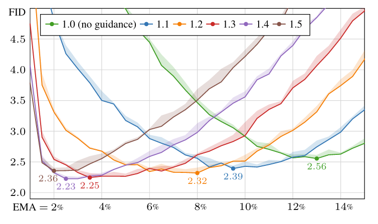
- Analysis

• Post-hoc EMA를 사용하여 EMA length에 따른 효과를 분석해 보면:
  • 아래 그림과 같이 각 $\texttt{Config}$ 마다 최적의 EMA length는 다르게 나타남
    - BUT, optimum의 narrowness는 각 weight tensor가 prefer 하는 EMA length에 대해 uniform 하게 나타남
  • 추가적으로 EMA length는 training이 진행됨에 따라 longer EMA로 slowly shift 함

EMA Length 별 효과

4. Experiments

- Settings

• Dataset : ImageNet
• Comparisons : EDM, ADM, VDM++, RIN

- Results

• 전체적으로 EDM2의 성능이 가장 우수함

Model 성능 비교

• Optimal EMA length는 guidance strength에 크게 의존함
  - 즉, vanilla/guidance 간의 discrepancy는 non-optimal EMA parameter로 인해 발생함

Guidance Strength 별 EMA Length

• EDM2는 latent diffusion 뿐만 아니라 RGB-space diffusion에서도 우수한 성능을 보임

RGB-Space Diffusion