[Paper 리뷰] LiteASR: Efficient Automatic Speech Recognition with Low-Rank Approximation

LiteASR: Efficient Automatic Speech Recognition with Low-Rank Approximation

---

• Automatic Speech Recognition model은 encoder-decoder architecture로 인해 computationally-intense 함
• LiteASR
  • Encoder에 Low-Rank Compression을 적용하여 transcription accuracy를 maintain 하면서 inference cost를 절감
  • Small calibration dataset을 활용하여 Principal Component Analysis를 적용하여 Linear transformation을 Low-Rank Matrix Multiplication chain으로 approximate
• 논문 (EMNLP 2025) : Paper Link

---

1. Introduction

• Whisper와 같은 Automatic Speech Recognition (ASR) system은 encoder-decoder architecture를 따름
  • BUT, ASR system은 long input sequence에 대해서는 computationally-intensive 함
    - 대표적으로 Whisper-Large-V3는 1.6B parameter를 가짐
  • 이로 인해 on-device, data-centered environment에서 ASR model을 활용하기 어려움

Encoder Size 별 Model 성능 비교

-> 그래서 기존 ASR system의 efficiency를 향상한 LiteASR을 제안

 

• LiteASR
  • Principal Component Analysis (PCA)를 통해 dominant component를 추출하고 rank-$k$ projection을 사용해 linear transformation을 approximate
  • 각 weight matrix를 2개의 low-rank matrix product로 decompose 하여 FLOPs를 절감
    
  • 추가적으로 self-attention mechanism을 modify 하여 optimization을 수행

< Overall of LiteASR >

• Low-Rank approximation을 활용한 efficient ASR model
• 결과적으로 기존보다 더 적은 parameter로 더 나은 ASR 성능을 달성

2. Method

• LiteASR은 서로 다른 layer의 activation으로부터 low-rank feature를 추출하여 ASR encoder를 compress 함
  - 이를 위해 calibration data를 사용하여 activation을 analyze 한 다음, model의 dense matrix multiplication을 low-rank matrix의 product로 convert 함

- Analyzing Activations in Transformers

• Weight matrix $W\in\mathbb{R}^{D_{in}\times D_{out}}$, bias vector $b\in\mathbb{R}^{D_{out}}$에 대해
  • 다음과 같이 정의되는 linear layer를 고려하자:
    (Eq. 1) $Y=XW+b$
    - 여기서 input activation $X\in \mathbb{R}^{L\times D_{in}}$은 forward pass를 통해 output activation $Y\in\mathbb{R}^{L\times D_{out}}$을 생성함
    - $D_{in}, D_{out}$ : 각각 input, output dimension, $L$ : sequence length
  • Activation distribution을 analyze 하기 위해, 논문은 $N_{calib}$ input으로 구성된 calibration data를 활용하여 해당 resulting output $Y$를 얻음
    - 즉, resulting dataset $Y$는 $L\times N_{calib}$ sample을 가지고 각 sample은 $D_{out}$-dimensional vector와 같음
  • 해당 calibration dataset에 대해, 논문은 observed activation을 Principal Component에 project 하는 것을 목표로 함
    1. 먼저 $Y_{M}\in\mathbb{R}^{D_{out}}$을 dataset $Y$의 mean vector라고 하자
    2. Standard PCA procedure에 따라 mean-centered data에 Singular Value Decomposition (SVD)를 적용하면:
       (Eq. 2) $U,S,V=\text{SVD}(Y-Y_{M})$
       - $V\in \mathbb{R}^{D_{out}\times D_{out}}$ : right singular vector의 matrix
    3. $V$의 first $k$ column을 select 하면 $V_{k}\in\mathbb{R}^{D_{out}\times k}$와 같이 나타낼 수 있고, 이를 통해 top-$k$ principal component를 capture 할 수 있음
    4. 결과적으로 original activation은 다음과 같이 approximate 됨:
       (Eq. 3) $ Y-Y_{M}\approx (Y-Y_{M})V_{k}V_{k}^{\top}$
       - 해당 approximation은 $Y$의 most significant feature를 retain 하면서 dimensionality를 reduce 함

Latency 비교

- Compressing Model Layers

• (Eq. 3)의 PCA approximation을 활용하여 original linear layer $Y=XW+b$를 low-rank matrix multiplication의 combination으로 rewrite 할 수 있음
  • $Y=XW+b$에 (Eq. 3)을 대입하면:
    (Eq. 4) $Y-Y_{M}\approx (XW+b-Y_{M})V_{k}V^{\top}_{k}$
    $\,\,\,\,\,\,\,\,\,\,\,\,\,\,\,\,\,\,\,\,\,\,\,\,\,\,\,\,\,\,\,\,\, Y\approx (XW+b-Y_{M})V_{k}V^{\top}_{k}+Y_{M}$
  • 이는 다음과 같이 reorganize 할 수 있음:
    (Eq. 5) $Y\approx X(WV_{k})V_{k}^{\top}+\left(Y_{M}+(b-Y_{M})V_{k}V^{\top}_{k}\right)$
  • 해당 factorization에서 original layer는 다음과 같이 decompose 됨:
    1. Weight matrix $WV_{k}\in\mathbb{R}^{D_{in}\times k}, V_{k}^{\top}\in\mathbb{R}^{k\times D_{out}}$을 가지는 2개의 low-rank linear transformation
    2. $Y_{M}+(b-Y_{M})V_{k}V^{\top}_{k}$로 주어지는 constant bias term
  • 해당 weight matrix, bias 모두 calibration data를 사용해 pre-compute 될 수 있으므로, $k$가 original dimension 보다 작을 때 해당 decomposition을 FLOPs를 크게 reduce 할 수 있음 

- How to Choose $k$

• $k$ value는 accuracy와 efficiency 간의 trade-off를 결정함
  - Smaller $k$는 aggressive approximation을 통해 efficiency를 향상할 수 있지만, accuracy loss가 나타남
• Accuracy Constraint
  • Accuracy를 preserve 하기 위해서는, top-$k$ principal component가 total variance의 sufficient portion을 capture 할 수 있어야 함
  • $S\in \mathbb{R}^{D_{out}}$을 mean-centered activation의 SVD로 얻어지는 singular value라고 하자
  • 그러면 다음을 enforce 할 수 있음:
    (Eq. 6) $\sum_{i=1}^{k}S_{i}^{2}>\theta\sum_{i=1}^{D_{out}}S_{i}^{2}$
    - $\theta$ : accuracy/efficiency 간의 trade-off를 control 하는 threshold (즉, data compression 정도)
• Efficiency Constraint
  • Original linear layer는 matrix multiplication에 대해 $\mathcal{O}(LD_{in}D_{out})$의 FLOPs를 요구함
    - 반면 (Eq. 4)의 decomposed form은 $\mathcal{O}(LD_{in}k+LkD_{out})$의 FLOPs를 요구함
  • 따라서 해당 approximation을 통해 computation reduction을 달성하기 위해서는
    1. 다음을 고려해야 함:
       (Eq. 7) $LD_{in}k+LkD_{out}<LD_{in}D_{out}$
    2. 이를 simplify 하면:
       (Eq. 8) $k(D_{in}+D_{out})<D_{in}D_{out}$
  • 실제로 Whipser-Large-V3에서 self-attention layer dimension은 $(D_{in},D_{out})=(1280,1280)$이고, MLP layer dimension은 $(1280,5120), (5120,1280)$과 같음
    - 즉, efficiency constraint는 self-attention에 대해 $k<640$, MLP layer에 대해 $k<1024$로 설정됨
• Practical Considerations
  • GPU efficiency를 향상하기 위해 논문은 $k$를 $16$의 배수로 restrict 함
    - 즉, (Eq. 6), (Eq. 7)을 모두 만족하는 $16$의 최소공배수를 $k$로 choice 함
  • $\theta$의 경우 $0.99$와 $0.999$ 사이의 값을 사용했을 때 accuracy, efficiency 간의 balance를 얻을 수 있음

Low-Rank Approximation

- Optimizing Self-Attention

• 추가적으로 self-attention layer를 optimize 할 수 있음
  - 특히 rank $k$가 per-head dimension 보다 작다면, FLOPs requirements를 줄이면서 mathematical operation을 preserving 하기 위해 attention score/value projection을 대체할 수 있음
• Standard Self-Attention
  • Multi-head attention에서 $h$를 head 수, $D_{head}$를 dimension-per-head 수라고 하면, total model dimension은 $D_{head}\times h$와 같음
  • $i$-th head에서 input activation matrix $X\in\mathbb{R}^{L\times D_{in}}$이 주어지면, self-attention mechanism은 3가지 linear projection을 수행함:
    (Eq. 9) $Q_{i}=XW_{Q}^{i},\,\,\,K_{i}=XW^{i}_{K},\,\,\,V_{i}=XW^{i}_{V}$
    - $W_{Q}^{i},W^{i}_{K},W^{i}_{V}\in\mathbb{R}^{D_{in}\times D_{head}}$ : weight matrix
    
  • 그러면 standard attention output은:
    (Eq. 10) $\text{Attention}(Q_{i},K_{i},V_{i})=\text{softmax}\left(\frac{Q_{i}K^{\top}_{i}}{\sqrt{D_{head}}}\right)V_{i}$
    - 여기서 $\text{softmax}$는 row-wise로 적용됨
• Attention Score Computation
  • Low-Rank approximation을 사용하여 각 projection을 factorize 하면:
    (Eq. 11) $Q_{i}=(XW_{Q_{1}})W^{i}_{Q_{2}}+b^{i}_{Q}$
    $\,\,\,\,\,\,\,\,\,\,\,\,\,\,\,\,\,\,\,\,\,K_{i}=(XW_{K_{1}})W_{K_{2}}^{i}+b_{K}^{i}$
    $\,\,\,\,\,\,\,\,\,\,\,\,\,\,\,\,\,\,\,\,\,V_{i}=(XW_{V_{1}})W_{V_{2}}^{i}+b_{V}^{i}$
    - $W_{Q_{1}}\in\mathbb{R}^{D_{in}\times k_{Q}}, W_{Q_{2}}^{i}\in\mathbb{R}^{k_{Q}\times D_{head}}, b_{Q}^{i}\in\mathbb{R}^{D_{head}}$ : low-rank approximation 이후의 $i$-th head에 대한 parameter
    - $k_{Q},k_{K},k_{V}$ : rank size
  • $A=XW_{Q_{1}}, B=XW_{K_{1}}$으로 두고 $Q_{i}K^{\top}_{i}$의 product를 expand 하면:
    (Eq. 12) $Q_{i}K_{i}^{\top}=\left(AW_{Q_{2}}^{i}+b_{Q}^{i}\right)\left(BW_{K_{2}}^{i}+b_{K}^{i}\right)^{\top}$
    $\,\,\,\,\,\,\,\,\,\,\,\,\,\,\,\,\,\,\,\,\,\,\,\,\,\,\,\,\,\,\,\,\,\,\,\,\,\,\,=\left(AW_{Q_{2}}^{i}+b_{Q}^{i}\right)\left(W_{K_{2}}^{i\top}B^{\top}+b^{i\top}_{K}\right)$
    $\,\,\,\,\,\,\,\,\,\,\,\,\,\,\,\,\,\,\,\,\,\,\,\,\,\,\,\,\,\,\,\,\,\,\,\,\,\,\,=AW_{Q_{2}}^{i}W_{K_{2}}^{i\top}B^{\top}+AW_{Q_{2}}^{i}b_{K}^{i\top} +b_{Q}^{i}W_{K_{2}}^{i}B^{\top}+ b_{Q}^{i}b_{K}^{\top}$
    - 해당 expansion에서 $AW_{Q_{2}}^{i}W^{i \top}_{K_{2}}B^{\top}$ term이 computational cost의 대부분을 차지하고, 나머지 term은 bias contribution을 나타냄
  • (Eq. 10)의 standard approach는 $Q_{i}, K_{i}^{\top}$을 separately compute 하고 multiply 하므로 $\mathcal{O}(L^{2}D_{head})$ FLOPs를 요구함
    1. 반면, (Eq. 12)는 smaller matrix product $W_{Q_{2}}^{i}W_{K_{2}}^{i\top}$을 compute 한 다음, $A,B$를 multiply 하므로 computational cost를 $\mathcal{O}(L_{k_{Q}}k_{K}+L^{2}\min(k_{Q},k_{K}))$로 줄일 수 있음
       - 즉, $\min(k_{Q},k_{K})<D_{head}$이면 (Eq. 12)가 더 efficient 함
    2. 따라서 논문은 sufficiently small rank에 대해 (Eq. 12)를 적용함
• Value Projection
  • Attention score matrix를 compute 하면:
    (Eq. 13) $S_{i}=\text{softmax}\left(\frac{Q_{i}K_{i}^{\top}}{\sqrt{D_{head}}}\right)\in\mathbb{R}^{L\times L}$
  • Final output은 $S_{i},V_{i}$를 multiply 하여 얻어짐:
    (Eq. 14) $S_{i}V_{i}=S_{i}\left((XW_{V_{1}})W_{V_{2}}^{i}+b_{V}^{i}\right)$
    $\,\,\,\,\,\,\,\,\,\,\,\,\,\,\,\,\,\,\,\,\,\,\,\,\,\,\,\,\,\,\,\,\,=S_{i}(XW_{V_{1}})W_{V_{2}}^{i}+S_{i}b_{V}^{i}$
  • 일반적으로 $(XW_{V_{1}})W_{V_{2}}^{i}$를 compute 한 다음, $S_{i}$를 multiply 하면 $\mathcal{O}(L^{2}D_{head}+Lk_{V}D_{head})$ FLOPs가 필요함
    - BUT, $S_{i}(XW_{V_{1}})$을 먼저 compute 하면 $\mathcal{O}(L^{2}k_{V}+Lk_{V}D_{head})$ FLOPs가 소모되므로 $k_{V}<D_{head}$일 때 더 efficient 함
  • 특히 $S_{i}$의 각 row의 합이 $1$이므로, bias term을 simplify 할 수 있음:
    (Eq. 15) $S_{i}b_{V}^{i}=b_{V}^{i}$
  • 결과적으로 value projection은 다음과 같이 rewrite 됨:
    (Eq. 16) $S_{i}V_{i}=\left(S_{i}(XW_{V_{1}})\right)W_{V_{2}}^{i}+b_{V_{1}}^{i}$
    - $k_{V}<D_{head}$인 경우 efficient 함
• Implementation
  • (Eq. 12), (Eq. 16)의 operation을 efficiently execute 하기 위해 논문은 Triton kernel을 사용하여 specialized kernel을 구성함
  • 해당 kernel은 FlashAttention을 extend 하여 computation을 optimize 함

3. Experiments

- Settings

• Dataset : VoxPopuli (VP), AMI, Earnings-22 (E22), GigaSpeech (GS), LibriSpeech (LS-C/LS-O), SPGISpeech (SG), TED-LIUM (TED)
• Comparisons : Whisper

- Results

• 전체적으로 LiteASR은 더 작은 parameter size로 더 우수한 WER을 달성함

Model 성능 비교

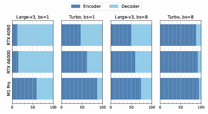
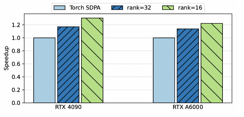
• Efficiency Evaluation
  • Inference speed 측면에서도 LiteASR이 가장 빠름

Speed 비교

• $32$ rank는 $14\%\text{~}17\%$, $16$ rank는 $22\%\text{~}30\%$의 acceleration이 가능함

Triton Kernel Performance

• Compression Ratio per Layer
  • Ealier layer는 substantial compression을 allow 함

Compression Ratio

• Sensitivity to $\theta$
  • $\theta$가 증가함에 따라 WER은 개선되고, $\theta=0.999$일 때 최적의 성능을 달성함

$\theta$의 영향

• Sensitivity to Languages
  • LiteASR은 다른 language에 대해서도 robust 한 성능을 보임

Language 별 성능

• Sensitivity to Models
  
  • WER 저하를 최소화하면서 encoder size를 $10\%$ 줄일 수 있음

Encoder Size 비교