[Paper 리뷰] APNet: An All-Frame-Level Neural Vocoder Incorporating Direct Prediction of Amplitude and Phase Spectra

APNet: An All-Frame-Level Neural Vocoder Incorporating Direct Prediction of Amplitude and Phase Spectra

---

• Amplitude와 Phase spectra를 직접 예측하여 acoustic feature로부터 음성 waveform을 재구성하는 neural vocoder
• APNet
  • Amplitude Spectrum Predictor (ASP)와 Phase Spectrum Predictor (PSP)로 구성
  • ASP는 acoustic feature로부터 frame-level amplitude spectra를 예측
  • PSP는 acoustic feature로부터 frame-level phase spectra를 예측
• 논문 (TASLP 2023) : Paper Link

---

1. Introduction

• Text-to-Speech (TTS)에서 acoustic model과 vocoder는 핵심적인 구조임
  • Acoustic model은 text에서 acoustic feature로의 mapping을 수행
  • Vocoder는 mel-spectrogram과 같은 acoustic feature로부터 음성 waveform을 재구성하는 역할
    - BUT, 기존의 vocoder는 spectral detail과 phase information에 대한 손실 문제가 있음
• Vocoder에서 합성 품질과 추론 효율성은 주요한 평가 기준임
  • Neural vocoder의 등장으로 통해 음성 합성 품질은 크게 개선됨
  • Autoregressive model : 기존 vocoder에 비해 높은 합성 품질을 달성했으나 여전히 느린 추론 속도를 보임
  • Knowledge-distilling-based / Flow-based / Glottis-based model : autoregressiv model에 비해 추론 효율성을 크게 개선했으나 여전히 높은 계산 복잡성을 보임
  • Neural source-filter (NSF) / GAN-based model : 최종 waveform을 직접적으로 예측하므로 여전히 느린 추론 속도
• 음성 waveform은 amplitude와 phase spectra로 상호변환 될 수 있으므로, 입력 acoustic feature의 waveform 대신 amplitude와 phase spectra를 예측하는 것으로 neural vocoder를 구성할 수 있음
  • ISTFTNET : HiFi-GAN의 middle layer에서 amplitude와 phase spectra를 추출해 ISTFT를 통해 최종 waveform을 합성
    - BUT, 낮은 sampling rate에서 amplitude와 phase를 효과적으로 예측하는데 어려움이 있음
  • HiNet : 계층적으로 amplitude와 phase를 예측하는 방법을 채택
    - BUT, phase wrapping 문제로 인해 NSF-like model이 추가적으로 필요함
  • Waveform의 raw amplitude와 phase spectra를 직접 예측하는 방식은 많이 연구되지 않음

-> 그래서 amplitude와 phase spectra에 대한 직접적인 예측을 활용하는 neural vocoder인 APNet을 제안

 

• APNet
  • Amplitude Spectrum Predictor (ASP)와 Phase Spectrum Predictor (PSP)로 구성
    - ASP와 PSP는 acoustic feature와 동일한 sampling rate로 raw amplitude와 phase를 예측한 다음, ISTFT를 통해 최종적인 waveform을 합성
    - ASP와 PSP를 비롯한 APNet의 모든 연산은 frame-level에서 수행되므로 높은 추론 효율성을 가짐
  • Amplitude spectra의 fidelity, Phase spectra의 precision, STFT의 consistency를 보장하고 최종 spectrum의 품질을 보장하기 위해 multi-level loss를 제시
    - 결과적으로 HiFi-GAN과 비슷한 합성 품질을 보이면서 14배 더 높은 추론 효율성을 달성

< Overall of APNet >

• Frame-level amplitude, phase 예측을 통해 추론 효율성을 향상하여 all-frame-level 음성 waveform 합성을 가능하게 함
• APNet의 parallel phase estimation architecture를 통해 까다로운 phase estimation에 대한 새로운 모델링 방식을 제시 

APNet과 다른 neural vocoder간의 구조 비교

2. Method

• APNet은 all-frame-level model로 sampling rate $F \cdot \frac{f_{s}}{T}$에서 동작
  1. APNet은 input acoustic feature (mel-spectrogram $M \in \mathbb{R}^{F\times 80}$)으로부터,
  2. raw sampling rate $F \cdot \frac{f_{s}}{T}$의 speech amplitude spectrum $\hat{A} \in \mathbb{R}^{F \times (N/2+1)}$과 phase spectrum $\hat{P} \in \mathbb{R}^{F \times (N/2+1)}$을 예측
  3. 이후 amplitude와 phase spectra는 STFT spectrum $\hat{S} \in \mathbb{C}^{F \times (N/2+1)}$로 reconstruct 됨
  4. 최종적으로 waveform $\hat{x} \in \mathbb{R}^{T}$는 ISTFT를 통해 복원됨
• APNet의 동작과정을 수식적으로 표현하면:
  • (Eq.1) $log \hat{A} = ASP(M)$
  • (Eq.2) $\hat{P} = PSP(M)$
  • (Eq.3) $\hat{S} = \hat{A} \cdot e^{j \hat{P}}$
  • (Eq.4) $\hat{x} = ISTFT(\hat{S})$

APNet의 개요

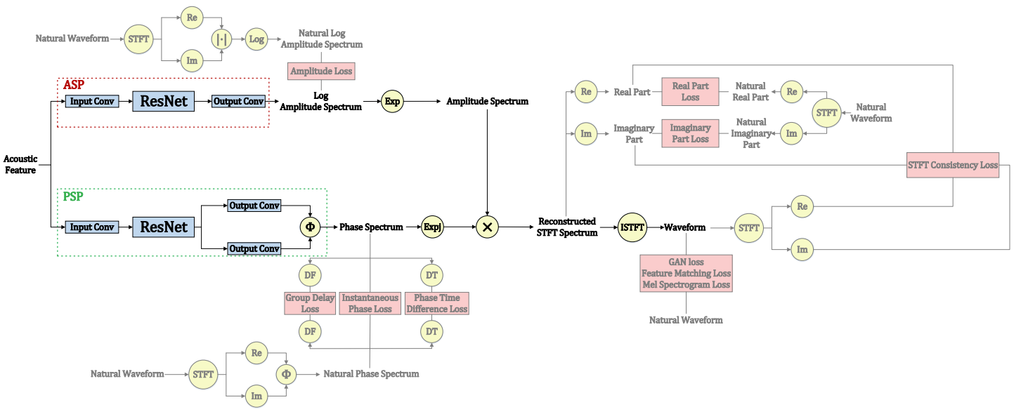
- Amplitude Spectrum Predictor

• Amplitude Spectrum Predictor (ASP)는 input acoustic feature로부터 log amplitude spectrum $log \hat{A}$를 예측 (Eq.1)
  • Input linear convolution layer, Residual convolution network, Output linear convolution layer로 구성
    - Residual convolution network는 $P$개의 parallel convolution block을 가짐
    - $P$개 block들의 output은 합산 및 평균되어 최종적으로 Leaky ReLU에 의해 activation 됨
  • $p$번째 block은 $Q$개의 residual convolution subblock (SubResBlock)을 concatenate 하여 구성

ASP와 PSP의 residual convolution network 구조

- Phase Spectrum Predictor

• Phase Spectrum Predictor (PSP)는 input acoustic feature로부터 phase spectrum $\hat{P}$를 예측 (Eq.2)
  • Input linear convolution layer, Residual convolution network, 2개의 Parallel output linear convolution layer, Phase calculation formula $\Phi$로 구성
    - Residual convolution network는 ASP의 구성과 동일
  • 2개의 Parallel output layer의 output을 $\tilde{R}, \tilde{I}$라고 하면,
    (Eq.5) $\hat{P} = \Phi(\tilde{R}, \tilde{I})$
    - $\hat{P}_{f,n} = \Phi(\tilde{R}_{f,n}, \tilde{I}_{f,n}), f=1,..., F, n=1,..., \frac{N}{2}+1$
    - $\hat{P}_{f,n}, \tilde{R}_{f,n}, \tilde{I}_{f,n}$ : 각각 $\hat{P}, \tilde{R}, \tilde{I}$의 요소
    - Phase의 범위 : $-\pi < \hat{P}_{f,n} \leq \pi$
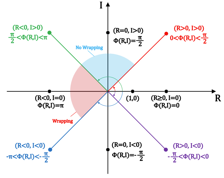
• Phase calculation formula $\Phi$의 유도
  • 두 개의 실수 $R \in \mathbb{R}, I \in \mathbb{R}$과 symbolic function을 아래와 같이 정의하자
    (Eq.6) $ Sgn^{*}(x)\left\{\begin{matrix} 1, x \geq 0  \\ -1, x < 0 \end{matrix}\right. $
  • 이때 Phase calculation formula $\Phi$는 2개의 변수를 가지고, $arctan(-\infty) = -\frac{\pi}{2}, arctan(+\infty) = \frac{\pi}{2}$ 이므로,
    (Eq.7) $\Phi(R,I) = arctan(\frac{I}{R}) - \frac{\pi}{2} \cdot Sgn^{*}(I) \cdot [Sgn^{*}(R)-1]$
    - $\Phi(0,0) = 0$, $\forall R \in \mathbb{R}, I \in \mathbb{R}, -\pi < \Phi(R,I) \leq \pi$
    - 출력되는 phase 값은 principal value interval $(-\pi, \pi]$ 내로 제한됨

Phase calculation formula $\Phi(R,I)$의 시각화

- Training and Inference Process

• Training 단계에서는 ASP, PSP 모두를 학습시키고 log amplitude spectra, phase spectra, 재구성된 STFT spectra, 최종 waveform에 대한 multi-level loss를 활용
  1. Log Amplitude Spectra Loss
     • 예측된 log amplitude spectra와 natural spectra를 일치시켜 고품질, high-fidelity의 log amplitude를 얻기 위함
     • Amplitude Loss : 예측된 log amplitude spectrum $log \hat{A}$와 natural amplitude $log A$ 간의 Mean Squared Error (MSE)
       : $L_{A} = E_{(log \hat{A}, log A)} \overline{(log \hat{A} - log A)^{2}}$
       - $\overline{X}$ : 행렬 $X$의 모든 값들의 평균
     • 이때 Natural log amplitude spectrum을 추출하기 위해서는, 먼저 natural speech wavefrom $x$에 STFT를 적용하여 STFT spectrum $S$를 얻음
       : $S = STFT(x; L, \frac{T}{F}, N)$
       - $L, \frac{T}{F}, N$ : 각각 frame length, frame shift, FFT point number
     • 이후 Natural log amplitude specturm은 아래와 같이 계산됨
       : $log A = log \sqrt{Re^{2}(S) + Im^{2}(S)}$
       - $Re, Im$ : 각각 실수부 계산, 허수부 계산 
  2. Phase Spectra Loss
     • Phase wrapping 문제를 극복하기 위해 사용되고, 예측된 phase spectra와 natural spectra를 일치시켜 phase apectra의 precision과 continuity를 향상
     • Instantaneous Phase Loss : 예측된 instantaneous phase specturm $\hat{P}$와 natural $P$ 사이의 negative cosine loss
       : $L_{IP} = -E_{(\hat{P}, P)} \overline{cos(\hat{P}-P)} $
       - Natural instantaneous phase spectrum은 Eq.7을 통해 아래와 같이 계산됨
       : $P = \Phi(Re(S), Im(S))$
     • Group Delay Loss : frequency bin의 phase variation을 반영하여 frequency별 phase의 음의 도함수로 정의됨
       - 이산 phase spectrum의 경우 group delay는 frequency 축을 따름
       - Group delay matrix를 아래와 같이 정의하면,
       : $W = [w_{1}, ..., w_{n}, ..., w_{\frac{N}{2}+1}]$
       : $w_{n} = \left [ \underset{1st}{0}, ..., 0, \underset{n-th}{1}, -1, 0, ..., \underset{(\frac{N}{2}+1-th)}{0} \right ]$
       - 따라서 $\hat{P}, P$에 대한 group delay loss는,
       : $\Delta_{DF}\hat{P} = \hat{P}W$
       : $\Delta_{DF}P = PW$
       - 최종적인 group delay loss는 예측된 group delay $\Delta_{DF}\hat{P}$와 natural $\Delta_{DF}P$ 간의 negative cosine loss로,
       : $L_{GD} = -E_{(\Delta_{DF}\hat{P}, \Delta_{DF}P)} \overline{cos(\Delta_{DF}\hat{P} - \Delta_{DF}P)}$
       -> Group delay loss는 frequency 축을 따라 natural과 예측된 phase 간의 continuity 차이를 줄임
     • Phase Time Difference Loss : time 축을 따라 natural과 예측된 phase 간의 continuity 차이를 줄임
       - Time difference matrix를 아래와 같이 정의하면,
       : $V = [v_{1}, ..., v_{f}, ..., v_{F}]^{T}$
       : $v_{f} = \left [ \underset{1st}{0}, ..., 0, \underset{f-th}{1}, -1, 0, ..., \underset{F-th}{0} \right ] ^{T}$
       - $\hat{P}, P$에 대한 time difference는,
       : $\Delta_{DT}\hat{P} = V\hat{P}$
       : $\Delta_{DT}P = VP$
       - 최종적인 phase time difference loss는 $\Delta_{DT}\hat{P}, \Delta_{DT}P$ 간의 negative consine loss로,
       : $ L_{PTD} = -E_{(\Delta_{DT}\hat{P}, \Delta_{DT}P)} \overline{ cos(\Delta_{DT}\hat{P}- \Delta_{DT}P)}$
     • 위 3가지 loss를 더해 최종적인 phase spectra loss로 사용
       : $L_{P} = L_{IP} + L_{GD} + L_{PTD}$
  3. Reconstructed STFT Spectra Loss
     • STFT spectrum domain $\mathbb{S}^{F \times (\frac{N}{2}+1)}$는 complex domain $\mathbb{C}^{F \times (\frac{N}{2}+1)}$의 subset이기 때문에 short-time spectral inconsistency issue가 존재함
       - Speech waveform $x \in \mathbb{R}^{T}$에 대해,
       : $S = STFT(x; L, \frac{T}{F}, N) \in \mathbb{S}^{F \times (\frac{N}{2}+1)}$
       : $ISTFT(S; L, \frac{T}{F}, N) = x$ 
       - 이때 reconstructed STFT spectrum $\hat{S} \in \mathbb{C}^{F \times (\frac{N}{2}+1)} - \mathbb{S}^{F \times (\frac{N}{2}+1)}$에 대해,
       : $\hat{x} = ISTFT(\hat{S}; L, \frac{T}{F}, N)$
       : $STFT(\hat{x}; L, \frac{T}{F}, N) = \tilde{S} \in \mathbb{S}^{F \times (\frac{N}{2}+1)} \neq \hat{S}$ 
       -> 즉, $\hat{S}$에 대응하는 consistent specturm은 $S$가 아닌 $\tilde{S}$이기 때문에 inconsistency 문제가 발생하여 reconstructed STFT spectrum $\hat{S}$를 신뢰할 수 없음
     • STFT Consistency Loss : short-time spectral inconsistency 문제를 해결하기 위해 $\hat{S}, \tilde{S}$ 간의 consistency를 계산
       : $L_{C} = E_{(\hat{S}, \tilde{S})} \overline { \{ [Re(\hat{S}) - Re(\tilde{S})]^{2} + [Im(\hat{S}) - Im(\tilde{S})]^{2} \} }$
     • Real and Imaginary Part Loss : $\hat{S}, S$의 실수부와 허수부에 대한 L1 distance의 평균으로 계산
       : $L_{R} = E_{(\hat{S}, S)} \overline { |Re(\hat{S}) - Re(S) | }$
       : $L_{I} = E_{ ( \hat{S},S)} \overline { |Im(\hat{S}) - Im(S) | }$
     • 위 3가지 loss를 더해 최종적인 reconstructed STFT spectra loss로 사용
       : $L_{S} = L_{C} + \lambda_{RI}L_{R} + \lambda_{RI}L_{I}$
  4. Waveform Loss
     • ISTFT를 통해 합성된 waveform $\hat{x}$와 natural waveform $x$간의 차이를 최소화하는 것을 목표로 함
     • HiFi-GAN의 loss와 동일하게 generator, discriminator loss $L_{GAN-G}, L_{GAN-D}$, feature matching loss $L_{FM}$, mel-spectrogram loss $L_{Mel}$로 구성
     • 최종적인 waveform loss는
       : $L_{W} = L_{GAN-G} + L_{FM} + \lambda_{Mel}L_{Mel}$
  5. Final Loss for training
     • APNet는 GAN의 학습방식을 따라 학습되며, 최종 loss는 위 loss들의 선형 결합으로 구성됨
       : $L_{G} = \lambda_{A}L_{A} + \lambda_{P}L_{P} + \lambda_{S}L_{S} + L_{W}$
       : $L_{D} = L_{GAN-D}$

STFT spectrum inconsistency issue에 대한 도식화

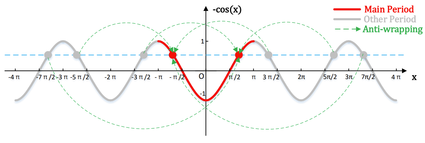
• Phase spectra loss 유도과정에서 사용된 negative cosine 함수는 아래 속성들로 인해 phase loss 정의에 적합한 성질을 가짐
  1. Parity
     • Negative cosine 함수는 phase difference의 절댓값에만 관심을 가지는 even function임
     • 예측된 phase는 방향에 관계없이 natural phase와 유사할 것을 기대하기 때문에 적합한 성질로 볼 수 있음
  2. Periodicity
     • Negative cosine 함수의 주기는 $2\pi$로 phase wrapping으로 발생하는 문제를 회피 가능
     • $\Phi(R,I)$ 시각화 그림에서, 파란색으로 표시된 부분 ($P^{no-wrapping}_{diff}$)과 빨간색으로 표시된 부분($P^{wrapping}_{diff})$의 phase difference의 절댓값은 동일함
       - BUT, 실제 계산에서는 빨간색으로 표시된 부분은 wrapping issue가 존재하기 때문에,
       : $|P^{no-wrapping}_{diff}| = 2\pi - |P^{wrapping}_{diff}|$
       - Negative cosine 함수를 적용하면,
       : $-cos(P^{no-wrapping}_{diff}) = -cos(P^{wrapping}_{diff})$
       -> 따라서 phase wrapping으로 인한 error를 방지하는 효과를 가짐
     • 아래 그림처럼 $L_{IP}, L_{GD}, L_{PTD}$를 계산할 때, negative cosine 함수는 $(-\pi, \pi]$ 외부의 값을 $(-\pi, \pi]$ 내부로 이동시키므로 anti-wrapping 역할을 수행함
  3. Monotonicity
     • Negative cosine 함수는 $[0, \pi]$에서 단조적으로 증가하므로 phase difference의 절댓값이 작을수록 loss의 크기도 작아짐

Negative Cosine 함수의 효과

3. Experiments

- Settings

• Dataset : LJSpeech
• Comparisons : HiFi-GAN, ISTFTNET, HiNet, MB-MelGAN

- Results

• SNR을 비롯한 정량적인 지표 측면에서는 APNet은 HiFi-GAN v2, ISTFTNET, HiNet, MB-MelGAN 보다 우수했지만, HiFi-GAN v1에 비해서는 낮은 성능을 보임
• MOS 측면의 주관적 평가에서는, APNet과 HiFi-GAN v1 간의 차이는 0.06으로 크게 차이 나지 않았고 ground truth의 MOS와 비슷한 품질을 보임
• RTF 측면에서, APNet은 GPU에서는 HiFi-GAN과 비슷한 속도를 보였으나 CPU만을 활용했을 때는 14배의 추론 속도 향상을 보임

비교 실험 결과

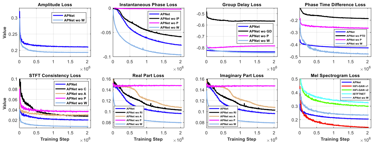
• LJSpeech dataset 학습과정에 대한 loss를 비교해 보면, 논문에서 제안된 multi-level loss가 정상적으로 수렴되는 것을 확인할 수 있음

Loss 비교 결과

• ABX test 결과를 살펴보면, APNet의 성능은 HiFi-GAN v1과는 크게 다르지 않았지만, HiFi-GAN v2와 ISTFTNET과 비교해보면 우수한 성능을 보임

ABX Test 결과

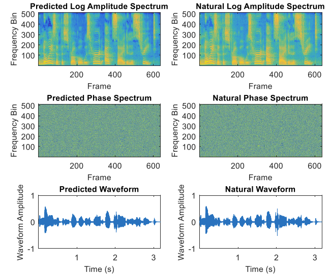
• ASP, PSP를 통해 예측된 log amplitude spectrum과 wrapped phase spectrum을 비교해보면 natural 음성과 비슷한 waveform으로 합성되는 것을 확인할 수 있음

ASP, PSP를 통한 합성 결과 비교

- Ablation Studies

• Phase estimation을 제거한 APNet wo PPEA와 APNet을 비교해보면, ABX test 측면에서는 당연하게도 APNet이 더 좋은 성능을 보임
• 각 loss들을 제거했을 때의 결과들과 비교해 보아도, APNet이 더 우수한 성능을 보임

APNet ablation에 대한 ABX test

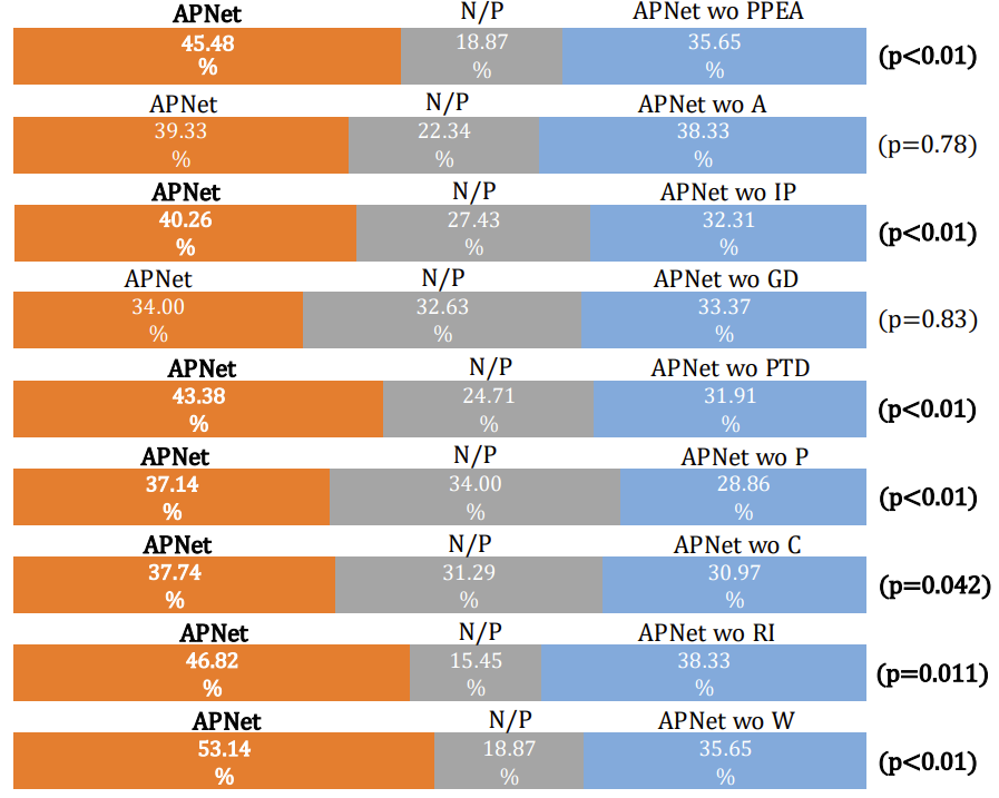
• 추가적으로 phase 관련 loss들을 제거하는 경우, 모든 정량적인 평가 지표가 급격히 저하되는 것으로 나타남

APNet ablation에 대한 정량적 지표 비교

• 생성된 음성의 spectrogram을 비교해 봤을 때 APNet wo A의 경우, high-frequency horizontal streak (파란색 박스)이 나타나는 것을 확인할 수 있음

생성된 음성의 Spectrogram 비교 1

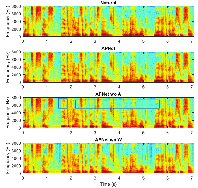
• Phase loss를 제거한 APNet wo PTD의 경우, 생성된 음성의 spectrogram을 비교해봤을 때, 저주파 영역에서 spectral blurring (초록색 박스)과 spectrual splitting (검은색 박스)가 발생함
  - Phase loss 제거로 인한 STFT spectrum의 incosistency 때문

생성된 음성의 Spectrogram 비교 2